Manual Information
Author(s): | V. Percuoco, D. Houpt |
Reviewer(s): | |
Revised by: | |
Management Approval: | |
Revised: | 376 | March 2018 |
Previous Versions: | V1.1 | 6 Jan 2014 (IODP-II), V1.0 | 7 August 2013 |
Domain: | Chemistry |
System: | ICP-AES Elemental Analysis |
Keywords: | ICP, dissolved metals |
Purpose a300pxnd Audience
This user guide is intended for use by scientists and technical staff who have laboratory experience with analytical instrumentation, preparing standards and samples, and data reduction; who have received an introduction and demonstration of the laboratory instrumentation aboard the JOIDES Resolution. Good laboratory practices and attention to laboratory safety are necessary while performing the procedures outlined in this user guide.
The user guide is to be used in conjunction with the Agilent 5100 and 5110 ICP-OES User’s Guide and the ICP Expert Help, both of which provide clear, detailed walkthroughs of instrument setup, operation, maintenance and troubleshooting procedures. Brief procedural videos are accessible through ICP Expert Help which demonstrate proper techniques when dealing with instrument components. The Agilent For Your Safety User’s Guide details additional safety information. Become acquainted with these resources before proceeding through this user guide.
Special Thanks
The JRSO wishes to thank Raymond M. Johnston and Jeff Ryan for their help and advice in fleshing out the solids methodology in this User Guide, as originally presented in the Exp. 366 IODP Proceedings Methods chapter. The JRSO also thanks Hans Brumsack for refining the interstitial water methodology as described on the Exp. 369 IODP Proceedings Methods chapter. The JRSO also thanks all of the many other geochemists who have provided help and advice over the many years of elemental analysis on the JOIDES Resolution.
Introduction and Theory of Operation
Inductively-coupled plasma optical emission spectrometry is a technique used to measure the elemental composition of a material by evaluating characteristic elemental spectra emitted during plasma heating. Dissolved sample flows through an introduction system in which the component molecules are desolvated, atomized and excited within an argon plasma. The transfer of energy from electronic and atomic collisions within the plasma excites elemental valence electrons across various atomic and ionic orbitals, which in turn release characteristic photons during electron de-excitation. Portions of these photons are directed through an optical chamber and ultimately fall upon a diffraction grating where they are reflected at angles determined by their wavelengths, separating them, like a prism, into discrete spectral orders. The photons impinge on an accurately aligned CCD or CMOS detector chip, and thus are mapped to a 2-D pixel array. A given element concentration is determined by locating its spectra within the array (i.e. on the chip), integrating the spectral intensity over a short time interval and comparing the results against a calibration curve of certified reference material.
The Agilent 5110 ICP-OES is used for routine shipboard measurement of interstitial water and hard rock matrices. The Waters method allows for simultaneous determination of major and minor dissolved elements. The Hard Rock method yields elements making up the major oxides, minor elements, and several trace metals that surpass the limits of detection. ICP-OES analytical results are heavily matrix dependent, thus the suite of elemental analytes may be altered on a per expedition basis depending upon the material collected.
Safety Considerations
Before conducting an analysis for the first time, consult the Agilent Technologies Agilent 5100 and 5110 ICP-OES User’s Guide and For Your Safety User’s Guide for a detailed review of safety issues. Listed below is a succinct overview of several important safety issues which are flagged, when appropriate, within the text:
- Ensure there is adequate storage space and ventilation for high-pressure argon gas bottles. Bottles must be secured to a rack, and the racks must be secured to the ship. The steel cap for each bottle must be in place whenever the bottles are not connected to the gas manifold. Use Swagelok Snoop Liquid Leak Detector to ensure proper seals at argon bottle and gas manifold connections.
- Samples and standards are made up in dilute solutions of concentrated nitric acid. Use proper PPE (nitrile gloves and eye protection) when handling acids. Always add acid to water. Be aware of the location of acid spill control and neutralization kits.
- Ensure the fume hood ventilation above the instrument is operational before igniting the plasma.
- The plasma torch is extremely hot during operation (6000 K). Do not handle the torch, RF coil, or other items within the torch compartment until ample time (>5 mins) has been given for the glassware to cool after operation. Wear heat resistant gloves if necessary.
The plasma emits ultraviolet and intense visible light. Ensure the torch compartment door is closed and sealed whenever igniting the plasma. Instrument safety interlocks will extinguish the plasma If the door is opened during operation, however, do not attempt to open the door while the plasma is active.
- Empty the waste container of acid residue after every batch analysis.
In This User Guide

Apparatus, Reagents and Materials
Hardware
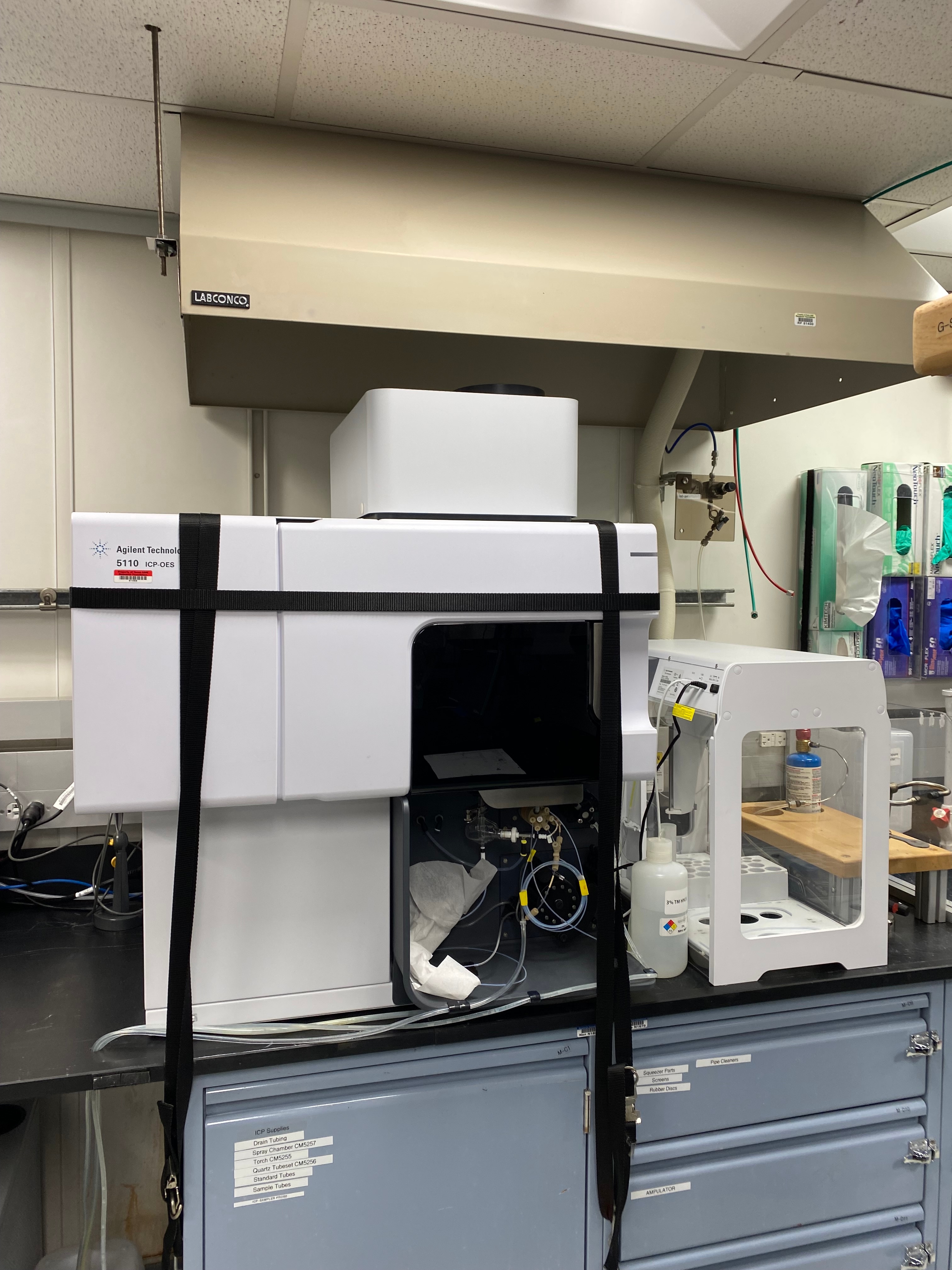
The complete Agilent 5110 ICP-OES system includes:
- Agilent 5110 Single View/Dual-View (SVDV) ICP-OES system equipped with the Automatic Valve Switching (AVS 6/7) option
- Agilent SPS4 4-rack autosampler
- Agilent G8481A Recirculating Chiller
- Mettler Toledo XS204 motion-compensated dual balance system
- Cahn Microbalance motion-compensated dual balance system
- Barnstead Reverse Osmosis Water Purification System
- Burrell Wrist-Action Shaker
- Thermolyne Muffle Furnace
Consumables
Reagents
- Reagent Water: 18 MΩ deionized water
- Sodium Chloride: Trace metal clean
- Nitric Acid (HNO3): Trace metal grade, 70% concentrated. Warning: Always add acid to water.
- Element Stock Solutions: Certified 1000 ppm: Al, Ba, Ca, Co, Cr, Cu, Fe, Ge, K, Mg, Mn, Na, Nb, Ni, P, Sc, Si, Sr, Ti, V, Y, Zn, Zr
- Element Internal Standards: Certified 1000 ppm: Be, In, Sb, Sc, Y
- Argon Gas: Ultra high purity (UHP) grade
- IAPSO standard seawater is produced to have a specific conductivity, K15, referenced to a known concentration of KCl at 15°C. It has been shown by Bacon et al. (2007) to be extremely consistent and stable over a reasonable period of time. It is assumed within this method that the concentration of the constituents in IAPSO standard seawater is, for all intents and purposes, the same as that of standard reference seawater. Using the numbers found in Millero (2008), substituting the averaged value for Gieskes (1991) and Summerhayes (1996) for lithium and alkalinity, the working concentrations are therefore:
Constituent1 | Concentration2 | Concentration3 | Concentration4 | Concentration5 | Working Concentrations |
Lithium (µM) | 27 | 25.7 | N/A | N/A | 26.4 |
Sodium (mM) | 480 | 480.2 | 480.2 | 480.7 | 480.7 |
Potassium (mM) | 10.44 | 10.46 | 10.46 | 10.46 | 10.46 |
Magnesium (mM) | 54 | 54.4 | 54.1 | 54.1 | 54.1 |
Calcium (mM) | 10.55 | 10.54 | 10.54 | 10.54 | 10.54 |
Strontium (µM) | 87 | 92 | 92.8 | 93.0 | 93.0 |
Chlorine (mM) | 559 | 559.6 | 559.4 | 559.6 | 559.6 |
Sulfate (mM) | 28.9 | N/A | 28.9 | 28.94 | 28.94 |
Alkalinity (mM) | 2.325 | N/A | 2.38 | N/A | 2.353 |
1. The molarity values in this table except for Gieskes et al. (1991) were calculated from the g/kg values in the reference using the density of standard seawater at 15°C (1.025 kg/L) in order to match the standardized K15 value for IAPSO seawater. 2. Gieskes et al. (1991) already given in terms of molarity. 3. Summerhayes et al. (1996); also quoted by the OSIL website as their reference for IAPSO constituents. 4. Pilson (1998). 5. Millero et al. (2008). N/A = not available from this author.
Methods for Preparation of Standards
Preparing Interstitial Water Standards
Preparing Reagents at the Start of Expedition
Prepare the following reagents at the beginning of an expedition and afterwards on an as-needed basis. For the relevant reagents listed below, the lithium carbonate (Li2CO3) is an optional addition.
- Internal Standards:
- Interstitial Waters: 100 ppm Be, In, Sc, 200 ppm Sb: Add 10 mL of each Be, In, Sc and 20 mL Sb elemental reference standards (1000 ppm) to a 100 mL volumetric flask, make up with 2% trace metal clean nitric acid. 100 mL is enough for 1000 samples
- Hardrock/Sediment: Same as the interstitial waters internal standard except no scandium (Sc) is added as it is present in rock/sediment matrices.
- Acidified Synthetic Seawater: 35 g trace metal clean NaCl + 29 mL concentrated trace metal HNO3 made up to 1 L with MQ water.
- Nitric Acid Solutions: Add 14.3 mL of concentrated trace metal HNO3 per 1 L of MQ water for each percentage point increase in concentration of acid solution (v/v), e.g. 1% HNO3: 14.3 mL, 2%: 28.6 mL, 3%: 43 mL HNO3. Warning: Always add acid to water.
- Rinse Solutions: Make 5-10 L at a time.
- Interstitial waters: 3% nitric (Use trace metal nitric acid)
- Hardrock/sediment: 10% nitric (Use trace metal nitric acid)
- Rinse Solutions: Make 5-10 L at a time.
- Matrix:
- Interstitial waters: 2% trace metal nitric
- Hardrock/sediment: 10% trace metal nitric, Optional: 53.25 g of ultrapure Li2CO3 may be added as an ionization buffer. Ensure the Li2CO3 is fully dissolved
Preparing the Calibration Standards
The calibration standards follow a matrix-matched internal standard approach that spans the range of expected concentrations of the pore water analytes. The recipe may need to be adjusted on a case-by-case basis. For the Interstitial Waters Method, two batches of standards must be prepared—a serial dilution of an in-house elemental cocktail and a serial dilution of IAPSO Seawater.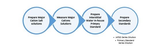
Preparing and Measuring Major Cation Salt Solutions:
Frequently, dissolved major cations increasing downhole surpass the upper bound of IAPSO concentrations and the certified 1000 ppm standards at working dilutions. These elements may be constrained within calibration curves by increasing the dynamic range of the calibration solutions with major cation salt doping. Primary salt solutions are prepared and concentrations are determined by ICP once at the beginning of an expedition and carried through further standard cocktails. There is no need to heat salts in the oven to desiccate. Note: magnesium chloride hexahydrate decomposes to magnesium tetrahydrate at 116.6°C:
- 1% Potassium: Make up 1.94 g of potassium chloride (KCl, 74.5513 g/mol) in 100 mL MQ water
- 1% Magnesium: Make up 9.13 g of magnesium chloride hexahydrate (MgCl2H12O6, 203.31 g/mol) in 100 mL MQ water
- 1% Calcium: Make up 3.8 g of calcium chloride dihydrate ( CaCl2H4O2, 147.008 g/mol) in 100 mL MQ water
- 3.5% NaCl: Acidified Synthetic Seawater reagent
Measure each solution against certified reference standards to acquire accurate concentrations for further standard dilutions.
- Working salt solutions: Pipette 1 mL of each 1% K, Mg, and Ca salt solution, and 286 µL of 3.5% NaCL into a single 100 mL volumetric flask and make up with 2% trace metal HNO3. With this solution, prepare 5-7 replicates of a 1:10 dilution (1 mL solution + 9 mL 2% HNO3) to be run by ICP. Vortex mix the aliquots. Each yields roughly a 10 ppm solution containing each major cation.
- Primary Certified Standard: Pipette 5 mL of each the 1000 ppm Ca, K, Mg, and Na standards into a 50 mL volumetric flask and make up with 2% trace metal HNO3.
Make up 6 calibration standards according to the following scheme:
Standard conc. (ppm) | Volume Primary Certified Standard (µL) | Volume 2% trace metal HNO3 (mL) |
Blank | 0 | 10 |
4 ppm | 400 | 9.6 |
8 ppm | 800 | 9.2 |
12 ppm | 1200 | 8.8 |
16 ppm | 1600 | 8.4 |
20 ppm | 2000 | 8.0 |
Use the template IODP_STANDARD_SALTSOLUTIONS_TEMPLATE to evaluate the 5-7 replicates against the above calibration standards. For each wavelength used, average the concentrations for the 5-7 replicates. Multiply the Ca, K, and Mg concentrations by a factor of 1000, and Na by a factor of 3500 to give the original 1% salt concentrations in ppm. In judging each element’s concentration, average all samples across all wavelengths after removing any erroneous/problematic lines. To start this analysis follow the steps given in Performing an ICP-OES Analysis. Adjust and update the concentrations of Na, Mg, Ca, and K listed in Table 1 to reflect the values measured in the 1% salt solutions.
Preparing Interstitial Water Working Standards:
Prepare a primary cocktail standard according to the recipe shown in columns 2 and 3 of Table 1. Pipette all individual standards into a single 100 mL volumetric flask and bring to volume with 2% trace metal HNO3. Na, Mg, Ca, and K values are from the major salt solutions which are determined in the preceding step, the remaining standards are 1000 ppm SPEX CertiPrep reference standards.
Table 1: Recipes of the primary cocktail and IAPSO (highlighted in blue) used to create working standards, and final concentrations of the working standards. Serially dilute the in-house cocktail and IAPSO according to the scheme given in Table 2. Na, Mg, Ca, and K are from the major salt solutions. Adjust concentrations accordingly. Iron and manganese values were excluded from IAPSO due to their low concentrations, and barium due to its precipitation with sulfate. Be wary of silicon concentrations in IAPSO due to its storage in glass containers.
|
|
|
| Final Concentrations of In-House Working Standards (uM) | ||||||||
Element | Primary CRM (ppm) | Volume (mL) | Cocktail (ppm) | 200 % | 100 % | 75 % | 50 % | 25 % | 10 % | 5 % | 1 % | 0 % |
B | 1000 | 3 | 30 | 5550 | 2775 | 2081 | 1387 | 693.7 | 277.5 | 138.7 | 27.75 | 0 |
Ba | 1000 | 5 | 50 | 728.2 | 364.1 | 273.1 | 182.0 | 91.02 | 36.41 | 18.20 | 3.641 | 0 |
Fe | 1000 | 0.5 | 5 | 179.1 | 89.5 | 67.15 | 44.77 | 22.38 | 8.953 | 4.477 | 0.8953 | 0 |
Li | 1000 | 0.5 | 5 | 1441 | 720.4 | 540.3 | 360.2 | 180.1 | 72.04 | 36.02 | 7.204 | 0 |
Mn | 1000 | 0.5 | 5 | 182.0 | 91.01 | 68.26 | 45.51 | 22.75 | 9.101 | 4.551 | 0.9101 | 0 |
P | 1000 | 0.5 | 5 | 322.9 | 161.4 | 121.1 | 80.71 | 40.36 | 16.14 | 8.071 | 1.614 | 0 |
Si | 1000 | 2.5 | 25 | 1780 | 890.1 | 667.6 | 445.1 | 222.5 | 89.01 | 44.51 | 8.901 | 0 |
Sr | 1000 | 5 | 50 | 1141 | 570.6 | 428.0 | 285.3 | 142.7 | 57.06 | 28.53 | 5.706 | 0 |
Na | ~13000 | 62 | 0 | |||||||||
Mg | ~10000 | 12 | 1200 | 98745 | 49373 | 37029 | 24686 | 12343 | 4937 | 2469 | 493.7 | 0 |
Ca | ~10000 | 4.5 | 450 | 22456 | 11228 | 8421 | 5614 | 2807 | 1123 | 561.4 | 112.3 | 0 |
K | ~10000 | 4 | 400 | 20461 | 10231 | 7673 | 5115 | 2558 | 1023 | 511.5 | 102.3 | 0 |
|
|
|
| Final Concentrations of IAPSO Working Standards (mM) | ||||||||
Element | IAPSO (ppm) | 200 % | 100 % | 75 % | 50 % | 25 % | 10 % | 5 % | 1 % | 0 % | ||
| Na | 10760 | 961.4 | 480.7 | 360.5 | 240.3 | 120.2 | 48.07 | 24.03 | 4.807 | 0 | ||
| Mg | 1293 | 108.3 | 54.14 | 40.60 | 27.07 | 13.53 | 5.414 | 2.707 | 0.5414 | 0 | ||
| Ca | 413 | 21.08 | 10.54 | 7.906 | 5.271 | 2.635 | 1.054 | 0.5271 | 0.1054 | 0 | ||
| K | 399 | 20.93 | 10.46 | 7.847 | 5.231 | 2.616 | 1.046 | 0.5231 | 0.1046 | 0 | ||
| S | 904 | 57.88 | 28.94 | 21.71 | 14.47 | 7.24 | 2.89 | 1.45 | 0.29 | 0 | ||
| Sr | 7.89 | 0.18 | 0.09 | 0.07 | 0.05 | 0.02 | 0.01 | 0 | 0 | 0 | ||
| Li | 0.202 | 0.06 | 0.03 | 0.02 | 0.01 | 0.01 | 0 | 0 | 0 | 0 | ||
| P | 0.07 | 0 | 0 | 0 | 0 | 0 | 0 | 0 | 0 | 0 | ||
| Si | 2.8 | 0.2 | 0.1 | 0.07 | 0.05 | 0.02 | 0.01 | 0 | 0 | 0 | ||
| B | 4.5 | 0.83 | 0.42 | 0.31 | 0.21 | 0.1 | 0.04 | 0.02 | 0 | 0 | ||
As listed in Table 2, create one set of working standards by making serial dilutions of the in-house synthetic cocktail (Table 1) using separate 100 mL volumetric flasks, adding the required amount of 3.5% sodium chloride, 100 ppm internal standard and bringing to volume with 2% trace metal HNO3. Prepare a set of IAPSO serial dilutions in the same fashion (do not add 3.5% sodium chloride). Note: Both sets of standards are analyzed in order to constrain Ba and S (predominately SO42-) which precipitate if present in the same vial (even if acidified), and to measure Na—which is necessarily kept constant to be used as an ionization buffer for the minor elements in the synthetic standards.
Table 2: Recipes for two sets of standard serial dilutions, one of the synthetic standard cocktail and the other of IAPSO. Prepare each standard in a 10 mL nalgene bottle, make up to volume with 2% trace metal nitric acid for IAPSO standards, and make up to volume with acidified synthetic seawater for In-House working standards. The final concentrations are listed in Table 1. Note: The left three columns indicate the recipe for the 10 ml In-House working standards and the three columns to the rights are the 10 ml IAPSO standards recipe.
In-House Working Standard Name | Volume In-House Cocktail (mL) | Volume Acidified 3.5% Seawater (mL) | Volume 100 ppm Internal Standard (mL) | IAPSO Working Standards | Volume | Volume 100 ppm Internal STD |
0% | 0 | 10 | 2 | 0% | 0 | 2 |
1% | 0.1 | 9.9 | 2 | 1% | 0.1 | 2 |
5% | 0.5 | 9.5 | 2 | 5% | 0.5 | 2 |
10% | 1 | 9 | 2 | 10% | 1 | 2 |
25% | 2.5 | 7.5 | 2 | 25% | 2.5 | 2 |
50% | 5 | 5 | 2 | 50% | 5 | 2 |
75% | 7.5 | 2.5 | 2 | 75% | 7.5 | 2 |
100% | 10 | 0 | 2 | 100% | 10 | 2 |
| 200% | 20 | 0 | 2 | 200% | 20 | 2 |
Alternate Method for Interstitial Water Standards
The aim of this method of preparing standards is to reduce error. Instead of standards and samples being prepared differently for analysis, they will all be prepared the same. In addition there will only be two solutions being pipetted for sample dilutions instead of three. This method also mimics prior methods used with the previous ICP where large batches of a matrix solution were made. Internal standard amounts were selected to remain close to the concentrations used in the above preparations.
- Matrix Solution: Pipette 2.25mL each of Be, In, Sc, and 4.5 mL Sb, along with 28.3 mL trace metal HNO3 to 1L of nanopure water.
| In-House Working Standard | Volume In-House Cocktail (mL) | Volume Acidified 3.5% Seawater (mL) | IAPSO Working Standards | Volume IAPSO (mL) | Volume 2% trace metal HNO3 (mL) |
|---|---|---|---|---|---|
| Acid Blank | 0 | 10 | |||
| 1% | .1 | 9.9 | 1% | .1 | 9.9 |
| 5% | .5 | 9.5 | 5% | .5 | 9.5 |
10% | 1 | 9 | 10% | 1 | 9 |
| 25% | 2.5 | 7.5 | 25% | 2.5 | 7.5 |
| 50% | 5 | 5 | 50% | 5 | 5 |
| 75% | 7.5 | 2.5 | 75% | 7.5 | 2.5 |
| 100% | 10 | 0 | 100% | 10 | 0 |
Preparing Hard Rock and Sediment Standards:
Hard rock and sediment standards are prepared according to the ICP-OES Hard Rock Preparation User Guide. Standards are fused with lithium metaborate (LiO2) at a 1:4 sample:flux ratio and then dissolved in a 10% trace metal HNO3 solution (Optional: doped with Li2CO3) for a total dilution factor of 1:2000. Lithium carbonate may be employed as an ionization buffer to maintain a relatively constant number of free electrons in the plasma to mitigate ionization and matrix effects and enhance peaks intensities of minor elements (not part of the routine analysis).
Major elements are reported in weight % (mass of oxide/mass of sample) of the respective oxide, with iron species being normalized to Fe2O3 (the designation Fe2O3t is used, where t = total). Minor elements are reported in units of ppm (mass of element/mass of sample).
An analytical procedural blank is prepared identically to the samples, with the exception that only 0.4 g of flux is fused and dissolved. An additional 0.1 g of flux is not added to mimic the TDS of the 0.5 g mix of sample + flux because this would provide an inaccurate quantitation of the impurities introduced by the amount of flux used in preparation of the unknowns.
Flux-Fusion Preparation of Rocks
Consult the IODP Hard Rock ICP Sample Preparation Guide for a complete, in-depth explanation of the hard rock and sediment sampling procedure. The amount of time necessary to prepare a single sample for analysis according to Table 4 is approximately 48 hours.
Table 3: ICP hard rock and sediment sampling and bead preparation timeline
Step | Time | Single (S) or Batch (B) |
Cutting the samples to size | 5 min | S |
| Cleaning the samples on the diamond wheel | 5 min | S |
Cleaning samples in methanol/DI | 30 min | B |
Drying samples | 12 hr | B |
Crushing samples in the X-Press | 15 min | S |
Grinding samples in the Shatterbox | 15 min | 3 samples |
Determining Loss-On-Ignition (LOI) | 20 hrs | B |
Making the sample beads | 15 min | S |
Diluting samples | 2 hrs | B |
Acid Cleaning Platinum Crucibles | 12 hrs | B |
Total | 48 hrs | B |
Dilution of Sediment/Hard Rock standards
Choose a suite of hard rock or sediment standards which matrix-match and span the range of expected concentrations within the samples. Consult Appendix 4: Table of Values for Hard Rock and Sediment Certified Reference Materials when choosing analytical standards. Standards are prepared in the same fashion as samples, as described in the proceeding section (see Hard Rock and Sediment (Solids Method)).
Characteristics of Flux Fusion Solutions
Flux fusion solutions become unstable over time; major and trace elements precipitate or form a gel, which is not always visible (since it is clear), so inspect solutions prior to analysis. The stability of the solution is proportional to the dilution factor and acid content and inversely proportional to the SiO2 content. A dilute solution is more stable than a concentrated one, and a solution becomes more stable with higher HNO3 presence. A flux-fusion solution enriched in SiO2 is likely to be more unstable than a basalt or shale solution. Analyze samples on the ICP shortly after they are dissolved.
Methods for Preparation of Samples
Interstitial Water (Waters Method)
This method applies to water samples in a 2% nitric acid solution at a 1:10 (v/v) dilution factor.
- Acidify pore water, rhizon or other aqueous samples with 5-10 uL of concentrated trace metal grade nitric acid and store refrigerated in sealed vials.
- When preparing an analytical batch, pipette 500 µL of sample (using an Eppendorf set-volume pipette) + 100 µL internal standard + 4.4 mL of matrix solution into a 15 mL vial. Cap and mix using a vortex stirrer for 10 seconds.
Interstitial Water (Alternate Method)
- Acidify pore water, rhizon or other aqueous samples with 5-10 uL of concentrated trace metal grade nitric acid and store refrigerated in sealed vials.
- When preparing an analytical batch, pipette 500 µL of sample or standard (using an Eppendorf set-volume pipette) + 4.5 mL of matrix solution into a 15 mL vial. Cap and mix using a vortex stirrer for 10 seconds.
Hard Rock and Sediment (Solids Method)
This method applies to hard rock and sediment samples in a 10% trace metal nitric acid solution at a 1:2000 (m/v) dilution factor
- Prime the 50 mL dispensette atop a 1 L bottle containing 10% nitric acid solution. Ensure there are no air bubbles present in the spigot.
- Add 50 mL of 10% nitric acid solution to a 125 mL HNO3 acid-cleaned Nalgene wide-mouthed bottle.
- Carefully place the sample bead (and all chipped pieces) in the 125 Nalgene bottle, close the lid, and agitate with the Burrell wrist-action shaker for 1 hr.
- Using a new or acid-washed 20 mL syringe, extract solution from the sample bottle and then using a 0.45 µm Acrodisc syringe filter, filter the solution into a 60 mL acid-cleaned Nalgene wide-mouth bottle. Repeat until the entire sample is filtered.
- Pipette 500 µL of the filtered solution into a 15 mL scintillation vial and dilute it with 100 µL hardrock internal standard + 4.4 mL dissolution solution. Cap and mix using a vortex stirrer for 10 seconds.
- Analyze samples within 48 hours of dilution.
Preparing an Analytical Sequence
Correct setup of the analytical sequence is integral to monitoring and troubleshooting the analytical results. Adhere to the following scheme in all cases:
- Bracket samples and with check standards. Use the 100% Level (IAPSO and the In-house) standards as checks. Prepare a large volume of the check standards in a volumetric flask and, after mixing, decant it into several aliquots to be analyzed intermittently every 8-10 samples.
- IMPORTANT: Analyze a blank before running the calibration standards, and periodically throughout a run. The blank must be diluted in the same fashion as the samples. It must contain the same amount of internal standard. The blank must be analyzed first.
- Analyze the standards at the beginning of a sequence. They can be in a random order.
- Always analyze the samples in a random order, do not sequence them by depth in hole.
Performing an ICP-OES Analysis
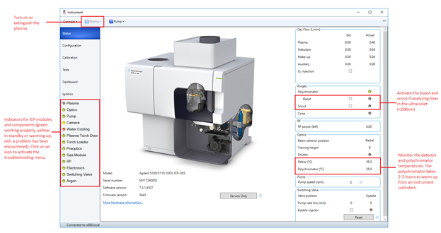
Figure 1: ICP Expert instrument dashboard.
Starting the Instrument
- Verify that the instrument is connected to the electrical mains (voltage requirement: 200 V), and that instrument is connected to the PC and network via Ethernet.
- Verify the Ar line is connected and the wall-mounted pressure gauge reads 90 psi. In the Upper Tweens ensure that two Ar gas manifold lines are each connected to a series of four Ar bottles. Open the manifold valve to only one set of four bottles. A fresh rack yields a pressure of ~2200-2400 psi—displayed on the pressure gauge connected in-line to the manifold above the Ar bottle racks. The regulator should be set around ~400 psi. The Ar usage is ~100 psi/hour with the plasma on, and ~2.5 psi/hr during standby. Use the Gas Status Monitor (http://eiger.ship.iodp.tamu.edu/GASSTATUS/) to monitor gas levels during an analysis. Note: Ar leaks may cause asphyxiation by displacing oxygen. Notify a coworker when manipulating gas lines in the Upper Tweens.
- Open the wall-mounted Ar valve above the ICP workstation.
- Power on the instrument by first enabling the kill-switch located on the rear-left, then press the power button located on the front-left of the instrument. The LED for the power button will flash green for a few seconds before steadying.
- Start the ICP Expert software.
- Wait approximately 30-45 minutes for the polychromator temperature to stabilize at 35.0°C. The temperature may periodically fluctuate by 0.1°C. If measuring wavelengths below 189 nm it is best to allow the polychromator to purge for a total time of 2-3 hours with Boost purge enabled.
- Turn on the water chiller. The default temperature setpoint should be at 20°C and the pressure setpoint at 59 psi. Turning on the instrument alone does not require the water chiller to be on, but you would want to have the chiller on for 30 minutes before igniting the plasma. The Peltier cooling temperature should be at -40°C.
- In ICP Expert click the ICP instrument button located on the top tool bar to bring up the instrument parameters menu. Click Plasma on. Over the next 60 seconds the plasma will ignite. If the plasma suddenly extinguishes during ignition, it is usually due to air drawn up through the tubing for the spray chamber rinse solution. Repeat this step while covering the end of the tubing with a gloved finger. The peristaltic pump comes on when the plasma ignites. Once the plasma is on, place the spray chamber rinse tubing in the 3% TM HNO3 bottle. Allow the plasma to stabilize for more than 20 minutes.
- Important: Ensure the peristaltic pump tubing is correctly seated. Place the tubing collars within the beams located above and below the pump wheel. Seat the collars within the beam grooves, not stretched along the outsides. Allow the pump to turn several times (enabling fast pump helps) for the tubing to work itself into position, then engage the pressure bars and if necessary adjust the tension of each. Bands of air or sample flowing through the lines leading to the pump should be unvarying in speed. If there is a chugging motion in fluid flow the pressure bars are too tight. If there is no flow, the pressure bars are too loose or there is blockage.
Selecting Elements, Wavelengths and Internal Standards to Measure
The ICP Expert software is designed in such a way that a method “template” may be set up and re-used for any number of subsequent analyses. When a run commences, the template file is converted to an ICP ExpertWorksheetFile (.esws)—which is identical to the template file except that it stores analysis results and archives instrument measurement conditions. It is important to keep in mind that all updates must be applied to the template file in order to be present in future runs. Altering the worksheet file (e.g. changing a calibration type, internal standard, removing or adding new lines, adjusting the standards table, etc) only applies to the respective worksheet.
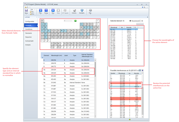 Figure 2: ICP Expert Elements Menu for selecting analytical lines and assigning internal standards
Specifying Instrument Measurement Conditions
A considerable amount of finesse is required to improve elemental results by changing the measurement conditions. By default, use the method developed on x369. It is stored under the name ICP-Template-Master on the ICP host PC. Table 5 lists the parameter values necessary to recreate the measurement conditions. If certain instrument components or parameters are changed, then all conditions must again be optimized as they are interlinked. In particular, adjust measurement conditions if:
- The sample isolation loop or any of the sample introduction lines are exchanged for one of different length and/or internal diameter.
- The pump rate is altered, or any time events are changed (e.g. valve uptake delay, rinse time, etc).
The number of condition sets changes from two, or SVDV is used.
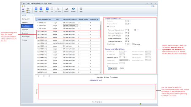
Figure 3: ICP Expert Conditions Menu for specifying instrument measurement parameters, assigning condition sets to individual lines, and setting integration areas. Note: These parameters cannot be changed once the sequence has started.Table 4: List of standard measurement parameters for ICP-OES analysis of interstitial water, sediment and hard rock. The first condition set to be run must include a 30 second plasma stabilization time, the plasma will remain stabilized for all subsequent condition sets provided the RF power and Ar flows are the same.
Parameter
Common Conditions
Condition Set 1
Condition Set 2
Replicates
3
Pump Speed (rpm)
12
Pump Rate –Uptake (mL/min)
28
Pump Rate –Inject (mL/min)
0.5
Valve uptake delay (s)
18.0
Bubble Injection Time (s)
2.0
Pre-emptive Rinse Time (s)
2.0
Rinse Time (s)
5
Read Time (s)
5
5
RF Power (kW)
1.20
1.20
Stabilization Time (s)
30
0
Viewing mode
Axial
Radial
Viewing Height (mm)
8
8
Nebulizer Flow (L/min)
0.70
0.70
Plasma Flow (L/min)
12.0
12.0
Auxiliary Flow (L/min)
1.00
1.00
Make up Flow (L/min)
0.00
0.00
Parameters for Common Conditions:
Replicates: The number of integrations for each condition set per sample.
Pump speed (rpm): The instrument peristaltic pump speed.
Pump rate – Uptake (mL/min): The rate at which sample is drawn through the sample isolation loop connected to the AVS.
Pump rate – Inject (mL/min): The rate at which sample is pumped into the nebulizer/spray chamber from the sample isolation loop.
Valve uptake delay (s): The length of time sample is pumped from the sample vial into and through the sample isolation loop.
Bubble injection time (s): The amount of time Ar is pumped into the sample isolation loop after sample uptake but before rinse uptake. This allows a bubble to separate the sample and standard within the uptake lines.
Pre-emptive Rinse Time (s):
Rinse time (s): The amount of time rinse solution is drawn through the sample lines after a sample uptake.
Parameters for Condition Sets
Read time (s): The length of time for a single replicate integration.
RF Power (kW): The forward power supplied by the RF coil to maintain the plasma.
Stabilization Time (s): The amount of time allotted for sample to be introduced from the AVS sample isolation loop to the plasma before performing integrations.
Viewing Mode: The angle from which the plasma is viewed. In “Axial” view the instrument views the plasma from the top facing downwards. In radial view, the instrument views the plasma from the side.
Viewing Height (mm): 8: The position of the radial optics when viewing the plasma from the side.
Nebulizer Flow (L/min): The argon flowrate introduced to the nebulizer which carries sample through the spray chamber
Plasma Flow (L/min): The argon flowrate introduced to the outer sheath of the torch in order to contain the plasma.
Aux flow (L/min): The argon flowrate introduced to the torch to maintain the plasma
Make up flow (L/min):
Creating a Standards Table
By following the standards dilution recipe given in this guide and using the default ICP Expert Templates (IODP_STANDARD_IW_MAJORS_MINORS_TEMPLATE.ests, IODP_STANDARD_HARDROCK_TEMPLATE_.ests), the standards table will not require major adjustment. In the case additional or different standards must be run:
- Click on the Standards menu located on the left side of the ICP Expert window
- Increase the Number of Standards to the desired quantities. Adjust the decimal places for the desired level of precision.
- Ensure Include Blank in Calibration is checked, and Correlation coefficient limit is set to 0.5000
- Within the table enter the standard names under Solution Label and enter the concentrations within the pertinent element columns. Attribute units to the concentrations by selecting from the dropdowns located immediately below the element header row.
- Adjust the “Calibration Fit” table so that the Calibration Error for each line is at 1000%. Uncheck Through Origin for each line.
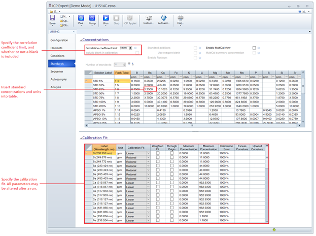
Figure 4: ICP Expert Standards Menu where the number and concentrations of analytical standards may be edited. The user may specify the type of calibration fit—which may be altered before, during and after an analysis
Creating a Sample Sequence
- Open the sample Sequence menu located on the left side of the ICP Expert window.
- Increase the Number of Samples to the desired quantity.
- In the sample table, enter the sample names and/or TextIDs and any dilution factors which deviate from the usual method dilution (dilution factors may likewise be adjusted after a run). Insert check standards every 8-10 samples. If necessary, change the values in the Rack:Tube column to designate each sample placement within the autosampler rack.
- Under the End of Run Actions, ensure the pump speed is set to 12 rpm and the rinse is set to 10 minutes.
- Next, open the Autosampler menu located below the Sequence menu. Notice the orientation of the autosampler displayed on the screen versus the autosampler placement on the countertop. Assign a rack for the standards by right-clicking on a rack, highlighting Rack Use and selecting Standards. Right-click on a single vial within the rack to set it as the Start Tube. Perform the same actions for samples by assigning sample racks and sample start tubes. The default rack types are 60 samples x 16 mm OD.
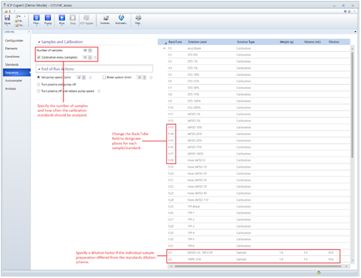
Figure 5: ICP Expert Sequence Menu for setting up a sample sequence and designating vial positions within the autosampler racks.
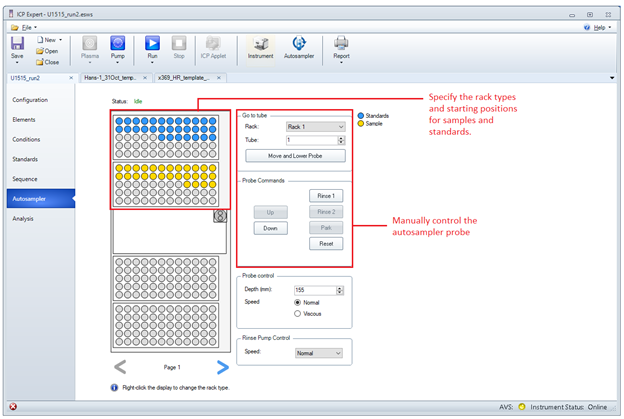
Figure 6: ICP Expert Autosampler Menu for assigning racks and vials to positions within the autosampler. The autosampler probe may be manually controlled from this menu.
Starting and Monitoring a Run
Within the Analysis menu, located on the lefthand side of the ICP Expert window (Figure 3), occasionally monitor the results during acquisition.
- Begin an analysis only after the standards and samples have been prepared and placed in the autosampler (with caps off), a standards table and sequence have been created in ICP Expert, and the correct measurement conditions have been applied on the Conditions tab. Press the Run button located on the top menu bar of ICP Expert. A message will appear asking to save the template as a worksheet file (.esws). Save to an expedition related data directory on the PC.
- As the instrument measures, periodically click on cells within the Results table to display the scan profile, calibration curve, and measurement statistics for each sample’s replicate integrations.
- In the spectrum window, move the dotted red vertical hash line so that it coincides with a peak maximum (Note: the adjustment propagates through all scans of the respective line). Ensure the entire peak is within the integration area. Click and drag the background points so there is minimal overlap with any spectral interferences. The type of background correction may be changed by right-clicking on the spectrum graph, highlighting Background fit and changing the selection.
- Ensure that the RSDs for each element are within the acceptable range. For values above the instrument detection limits, expect most RSDs to be below 1-2%. Values above but near the LOD will typically have an RSD of 5%, whereas values below the LOD will typically return RSD’s of 5%+. After measuring the standards, if there is a systematic increasing/decreasing trend in intensity for the three replicate integrations, stop the run and troubleshoot. (See Section Troubleshooting for help).
- Outliers may be removed by selecting a sample in the results table and unchecking the boxes for Replicate located on the pane at the bottom of the screen. The software disregards a sample/standard if all replicates are removed.
- If necessary, change the calibration type (linear, quadratic, rational) by navigating to the Standards menu and changing the selection within the Calibration Fit menu.
- On an element case-by-case basis, remove the replicates for high-end standards which greatly over range the sample concentrations.
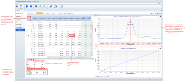
Figure 7: ICP Expert Analysis window. User may view analytical results during acquisition, dynamically change background corrections and integration areas, flag outliers, and view calibrations
Exporting, Vetting and Uploading Data
Follow the subsequent steps only after a run has completed, the calibrations have been verified, dilutions have been taken into account, values below LODs have been disregarded and results are ready for upload. Follow the guidelines in the Quality Assurance and Data Reduction section when vetting ICP-OES results.
- For each element wavelength in the results table, right-click on the column header, select Column Properties and toggle off all result flags (Figure 6).
- Left-click the empty cell on the left-most column of the Results table (left of the Rack:Tube header) to select all the results. Right-click the same cell then select “Export selected solutions.” Save the file to an expedition specific directory.
- Open the AIDR-ICP Data Reduction.xlsm. On the Raw Data worksheet open the user menu (CTRL+SHIFT+W) and select Import Data. Follow the prompts.
- Manually Copy the Condition Sets and Element Lists tables from ICP Expert to the appropriate tables located on the Condition Set and Element List tab in the Agilent Data Reduction Program. Open the user menu on the Raw Data worksheet and Format Data.
- (Optional) Download a curatorial report from LORE and paste it to the table on the Curatorial Report tab.
- On the Reduced Data tab, open the menu (CTRL+SHIFT+W) and click Refresh PivotTable.
- Use the slicers to filter out undesired elemental wavelengths. Porewater graphs may be generated by opening the menu and selecting Show Concentration Plots.
- At this point, pass the workbook over to the geochemists. After the data has been vetted, open the menu (CTRL+SHIFT+W) on the Reduced Data tab and select Spreadsheet Uploader Format. The data will be formatted for upload.
- Paste into Spreadsheet uploader, validate the sheet, then upload to LIMS. Data must be pasted into Spreadsheet Uploader in chunks of 500 rows or less.
Post-Run Shutdown and Cleanup
Instrument Shutdown Procedure
- Cycle the nitric acid rinse solution for 10 minutes, followed by DI water for 5 minutes, then remove the sample uptake tubing from solution and allow air to purge the lines and introduction system for 10 minutes or to dryness.
- Extinguish the plasma by clicking Plasma off from the ICP Expert menu.
- Disengage the peristaltic pump tubing on both the instrument and autosampler.
- After 10 minutes necessary for the RF coil to fully cool, switch off the water cooler.
- If another analysis will be conducted within the following week, leave the instrument on with Ar flowing (usage is ~2.5 psi/hr in standby). If it is the end of expedition or there will be a long interval between the next analysis, turn off the Ar gas inlet by closing the wall-mounted valve located above the instrument. Turn off the power using the switch on the front left, wait for the green LED to stop blinking, then turn off the mains power switch located on the rear left of the instrument.
- Leave the vials in the autosampler rack until the results have been inspected to ensure no two vials were misplaced during the analysis. Remove the labels from the vials, empty the contents into the waste container, and rinse the vials with tap water. Soak them in 10% HNO3 for 12 hours.
- If proceeding to an interstitial water analysis after performing a hard rock analysis change all the sample introduction tubing and glassware to prevent Li and B contamination. These include the autosampler probe, sample uptake tubing, sample introduction loop, nebulizer and spray chamber.
Cleaning Instrument Components:
Follow the routine cleaning procedure outlined in the Agilent 5100 and 5100 ICP-OES User’s Guide when cleaning or servicing any instrument components. Walkthrough videos and step-by-step instructions are accessible through the ICP Expert Help menu, underneath the “How to,” “Troubleshooting,” and “Maintenance” folders.
Daily Cleaning and Maintenance
- Check the torch for cleanliness. To clean the torch, soak the end in a small volume of 50% aqua regia. For 200 mL, combine 100 mL DI water, 25 mL of concentrated HNO3, and 75 mL of concentrated HCl in a glass beaker. Fresh aqua regia has a darkish orange-brown hue that gradually becomes lighter as the nitrogen degasses as nitrogen dioxide, at which point it should be replaced. Caution: Always add acid to water. Aqua regia is more corrosive than its components taken separately. Wear proper PPE, including a face shield and lab coat. Work in a fume hood. Store aqua regia in a glass or Teflon container as it will corrode regular LDPE or HDPE bottles.
- Inspect the elasticity of the peristaltic pump and AVS tubing, replace if necessary.
- Flush the sample flow paths with DI water to remove any acidic solution and ensure there are no blockages.
- Wrap the CRM bottle necks and caps in Parafilm to prevent evaporation.
Weekly Cleaning and Maintenance
- Clean the torch, cone, snout, spray chamber and nebulizer. Consult ICP Expert Help Menu for in-depth videos of removal, cleaning, and installation procedures.
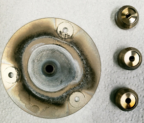
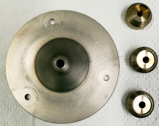
Figure 8: Cone before cleaning Figure 9: Cone after cleaning with a non-metal scouring pad in DI water.Figure 8: Cone before cleaning
Monthly Cleaning and Maintenance
- Clean the inlet filter for the cooling air
- Perform an ICP-OES calibration
- Remove and clean the water filter
- Inspect the axial and radial optics windows, replace if necessary
- Check the water level in the water chiller
- Clean the water chiller radiator of dirt and dust build-up
- Drain the water chiller and either refill or treat with algaecide
Data Available in LORE
Interstitial Waters Standard Report
- Exp: expedition number
- Site: site number
- Hole: hole number
- Core: core number
- Type: type indicates the coring tool used to recover the core (typical types are F, H, R, X).
- Sect: section number
- A/W: archive (A) or working (W) section half.
- Top offset on section (cm): position of the upper edge of the sample, measured relative to the top of the section.
- Bottom offset on section (cm): position of the lower edge of the sample, measured relative to the top of the section.
- Top depth CSF-A (m): position of observation expressed relative to the top of the hole.
- Top depth [other] (m): position of observation expressed relative to the top of the hole. The location is presented in a scale selected by the science party or the report user.
- Sampling tool: tool used to collect sample
- Data columns: header lists parameter measured and concentration units, followed by wavelength (for ICP-AES) and then analysis method.
Expanded ICPAES Report
- Exp: expedition number
- Site: site number
- Hole: hole number
- Core: core number
- Type: type indicates the coring tool used to recover the core (typical types are F, H, R, X).
- Sect: section number
- A/W: archive (A) or working (W) section half.
- text_id: automatically generated unique database identifier for a sample, visible on printed labels
- sample_number: sample number of sample. text ID with sample type prefix removed.
- label_id: id combining exp, site, hole, core, type, sect, A/W, parent sample name (if any), sample name
- sample_name: name of sample
- x_sample_state:
- x_project: expedition project the sample is uploaded under. typically the same as Exp.
- x_capt_loc:
- location: location sample was taken
- x_sampling_tool: tool used to collect sample
- changed_by: name of person who uploaded sample
- changed_on: date and time sample was uploaded
- sample_type: type of sample. typically LIQ, for liquid.
- x_offset: top offset of parent sample where sample was taken in m
- x_offset_cm: top offset of parent sample where sample was taken in cm
- x_bottom_offset_cm: bottom offset of parent sample where sample was taken in cm
- x_diameter:
- x_idmp:
- x_orig_len:
- x_length: length of sample in m
- x_lengeth_cm: length of sample in cm
- status:
- old_status:
- original_sample:
- parent_sample:
- standard:
- login_by: name of person logged into LIMS application used for this test
- sampled_date:
- legacy:
- test changed_on: date of last edit of analysis
- test date_started: date analysis was started
- test group_name:
- test status:
- test old_status:
- test test_number: unique number associated with the instrument measurement steps that produced these data
- test date_received: date analysis was uploaded to LIMS
- test instrument: instrument used to perform analysis
- test analysis: analysis type
- test x_project: project test was assigned to
- test version:
- test order_number:
- test replicate_test:
- test replicate_count:
- rest sample_number: sample number for sample the analysis was performed on
Top depth CSF-A (m): position of observation expressed relative to the top of the hole.
Bottom depth CSF-A (m): position of observation expressed relative to the top of the hole.
Top depth CSF-B (m):
Bottom depth CSF-B (m):
- batch_id:
- calibrated_name: element analyzed along with concentration unit
- calibration:
- concentration: measured concentration of analyzed element
- corrected_intensity:
- correlation:
- drift_asman_id:
- drift_corrected:
- drift_filename:
- element_conc_dissolved (uM)
- element_name: name of analyzed element
- ssup_asman_id: download link for the batch of data uploaded through spreadsheet uploader
- ssup_filename: filename of spreadsheet uploader batch
- view: view mode that analysis was performed in (axial, radial, svdv)
- wavelength: wavelength that element was measured at
sample description: observations recorded about the sample itself
test test_comment: observations about a measurement or the measurement process; some measurement observations may be under Result comments
result comments: observations about a measurement or the measurement process; some measurement observations may be under Test Comments
Note: Iron is expressed as Fe2O3t, or total Iron (III) oxide.
Quality Assurance/Quality Control and Data Reduction
Aside from performing drift corrections, the Agilent ICP Expert software accounts for all data reduction. The option to normalize to any analyzed internal standard wavelength is available before, during and after a run. Additionally, quality control specifications may be changed to flag troublesome data. The following quality controls ultimately fall under the purview of the geochemists.
Implement the following steps to vet the data:
- Ensure there are no spectral interferences overlapping the peaks of interest.
- If spectral interferences are present, inspect the interference level in the blank versus the level in the standards. If the interference is not constant between all standards, disregard the line.
- Ensure the linear/quadratic/rational relationship of each wavelength calibration curve.
- Ensure the sample concentrations are less than the greatest calibration point. Remove standards from the calibration which greatly over range elemental abundances in the samples as they may bias the calibration curve slope.
- Do not remove a point from the calibration unless:
- The RSD % is outside of the allowable.
- A student T-Test or Grubbs Outlier Test has been performed on the point. Use the signal intensity-to-concentration ratios to compare the point against the mean and standard deviation of the population of the other points making up the calibration curve.
- The liquid level of the vial in the autosampler rack indicates some sample volume was not introduced.
- For each line, verify that the accuracy (% difference) of any check standards is within tolerance.
- Ensure the % change in drift standards throughout the course of the analytical run is insignificant, or, if it is not, take into account drift with linear drift factors. If the drift is random (non-systematic), then ignore drift corrections and consider troubleshooting precision issues.
- Ensure there is not a significant deviation in the slopes of calibration curves as compared to the same curves in previous runs.
- Before uploading to LIMS, flag values below detection limit, higher than the highest calibration point, or have poor %RSD. AIDR has capabilities for this.
Sediment/Rock Standards
- For a given sample/standard, ensure that the total % recovery of major oxides is 100 ± 2 wt%.
- Periodically ensure that sediment and rock standard certified reference material values are up to date with the literature.
Troubleshooting
Plasma Extinguishes upon Startup:
This occurs when air contaminates the torch box or the torch is not dry. Verify the torch is dry. Allow Argon to purge the torch box for 10 minutes or so. When igniting the plasma, press a glove finger against the end of the rinse uptake tubing connected to the spray chamber to cut off it from drawing in air or solution.
Steps Going Forward for Method Improvement:
- Attempt to implement the SVDV dual view mode for simultaneous axial and radial measurement. This will reduce analysis time, argon usage, and the amount of pore water required per sample analysis.
- Adapt the current ICP Template by changing the number of condition sets to 1 (SVDV).
- Adjust the Common Conditions so there is at least a 30 second delay after sample initially reaches the torch for the plasma to stabilize. It is easiest to time this by running a sample containing sodium as it emits a bright orange color within the plasma.
- Adjust the pump conditions so that the sample isolation loop fills with enough sample for each replicate integration. Watch the fluids flow through the lines to aid in timing. If the measurement finishes before all the sample has been ejected from the sample loop, then on the next run increase the “Pre-emptive rinse time” so that rinse solution is drawn into the sample isolation loop in place of the tail-end volume of sample.
- After optimization, run a calibration curve. Ensure there are no systematic increases or decreases in intensities across each replicate. RSD should be below 2%. Inspect the calibration curves for linearity (or quadratic fits). The squared correlation coefficient must be greater than 0.90 in order to be acceptable.
- Compare spectral interferences for each element wavelength between the current Axial/Radial method and SVDV. Investigate the presence or absence of interferences and each interference intensity in relation to the analyte peak intensity. Calculate detections limits. Compile the data into a table and compare against the Axial/Radial method.
- Headers: Analytical Wavelengths
- Rows: Detection Limits, % RSD (low and high sample), % Accuracy (Low and High sample), squared correlation coefficient, calibration curve slope and intercept, dynamic range, internal standards used, spectral interferences.
- Attempt to optimize the RF forward power and viewing height parameters in Axial/Radial mode. This may improve analytical measurement and detection of minors elements such as Fe and P. Keep in mind that the plasma must stabilize for a period if the RF forward power is altered.
- Purchase and implement an Argon Humidifier to help reduce precipitate buildup in the nebulizer.
- Create a generic report template using the ICP report designer that includes all the measurement parameters, calibration information, sequence information, results and statistics using the ICP Expert Report Designer. Reports are exported as pdfs. Store the reports to Uservol and to the instrument host PC. Move towards implementing an uploader in MUT which captures reports.
- Create an Excel script (or other) to aid in quickly visualizing data downhole from the data exported after a run.
- Create an Excel script to apply a linear drift correction to select lines.
- Create a Database (Excel or other) which captures calibration information for future reference.
- Revisit whether or not sample/standard residues from LOI yield valid measurements, or instead, direct fluxing of standards before combustion should be performed.
- Certified reference materials are only valid for drying at 120°C.
- LOI is loss of H2O, CO2 but also gain of O2 from oxidation products, which complicates the final mass value
- Nearly 20 hrs of sample preparation time may be saved.
References
Agilent Technologies, ICP Expert Software, Version 7.3.1.9507, 2017
Agilent Technologies “Agilent 5100 and 5110 ICP-OES User’s Guide,” Manual # G8010-90002, October 2016, 4th Ed, Malaysia
Agilent Technologies “For Your Safety User’s Guide,” Manual # 5971-6636, February 2014, 2nd Ed, Malaysia
Agilent Technologies “Agilent SPS 4 Autosampler User’s Guide,” Manual # G8410-90000, May 2015 Revision A, Malaysia
Bacon, S., Culkin, F., Higgs, N., and Ridout, P., 2007. IAPSO standard seawater: definition of the uncertainty in the calibration procedure, and stability of recent batches. J. Atmos. Oceanic Technol., 24(10):1785–1799. doi:10.1175/JTECH2081.1
Gieskes, J.M., Gamo, T., and Brumsack, H., 1991. Chemical methods for interstitial water analysis aboard JOIDES Resolution. ODP Tech. Note, 15. doi:10.2973/odp.tn.15.1991
Houpt, D., 2013. Leeman Prodigy ICP-AES User Guide. International Ocean Discovery Program.
Millero, F.J., Feistel, R., Wright, D.G., and McDougall, T.J., 2008. The composition of Standard Seawater and the definition of the Reference-Composition Salinity Scale. Deep-Sea Res., Part. I, 55(1):50–72. doi:10.1016/j.dsr.2007.10.001
Murray, R.W., Miller, D.J., and Kryc, K.A., 2000. Analysis of major and trace elements in rocks, sediments, and interstitial waters by inductively coupled plasma–atomic emission spectrometry (ICP-AES). ODP Tech. Note, 29. doi:10.2973/odp.tn.29.2000
Pilson, M.E.Q., 1998. Major Constituents of Seawater. In: An Introduction to the Chemistry of the Sea. Upper Saddle River, NJ (Prentice Hall).
Skoog et al. 1992 Fundamentals of Analytical Chemistry 7th Ed.
Skoog et al. 1997 Principles of Instrumental Analysis 5th Ed.
Summerhayes, C.P., and Thorpe, S.A., 1996. Oceanography An Illustrated Guide, Chapter 11, 165–181.
Appendix 1: List of Instrument Measurement Parameters, Element Wavelengths and Internal Standard Wavelengths
The following tables detail analytical wavelengths, internal standards, and viewing modes for elements measured in the Hardrock/Sediment and Interstial Waters methods. Each table is followed by a list of similar line combinations, which have been rejected for various reasons listed in each table. An Excel spreadsheet (Hardrock-Sediment_Interstital Waters_Default Analytical Wavelengths Library.xlsx) containing this information is available on the desktop of the ICP host computer. If should be periodically updated as lines are added or removed.
Interstitial Waters Method:
Use the analytical lines, internal standards and torch views listed in Table 5 to recreate the default instrument condition set for analysis of dissolved elements in pore waters. These values are appropriate for the interstitial water dilution scheme given in the text above. Altering the dilution scheme by changing the concentrations of analytical standards or diluting samples and standards by a ratio other than 1:10, may affect the respective calibration curves, in which case, these conditions may need to be adjusted.
Table 5: List of instrument conditions to recreate the method for measurement of major and minor elements in interstitial water.
Element | Wavelength (nm) | Type | Internal Standard (Wavelength nm) | View |
B | 208.956 | Analyte | Sb (206.834) | Axial |
B | 249.678 | Analyte | Sb (206.834) | Axial |
B | 249.772 | Analyte | Sb (206.834) | Radial |
Ba | 230.424 | Analyte | Sb (206.834) | Axial |
Ba | 230.424 | Analyte | Sb (206.834) | Radial |
Ba | 455.403 | Analyte | Sc (424.682) | Axial |
Ba | 455.403 | Analyte | Sc (361.383) | Radial |
Be | 313.042 | Internal Standard | None | Axial |
Ca | 315.887 | Analyte | Sc (361.383) | Axial |
Ca | 315.887 | Analyte | Sc (361.383) | Radial |
Ca | 317.933 | Analyte | Sc (361.383) | Axial |
Ca | 317.933 | Analyte | Sc (361.383) | Radial |
Ca | 318.127 | Analyte | Sc (361.383) | Axial |
Ca | 318.127 | Analyte | Sc (361.383) | Radial |
Ca | 431.865 | Analyte | Sc (361.383) | Axial |
Ca | 431.865 | Analyte | Sc (361.383) | Radial |
Fe | 238.204 | Analyte | Sc (361.383) | Axial |
Fe | 238.204 | Analyte | Be (313.042) | Radial |
Fe | 239.563 | Analyte | Be (313.042) | Axial |
Fe | 239.563 | Analyte | Sc (361.383) | Radial |
Fe | 259.94 | Analyte | Be (313.042) | Axial |
Fe | 259.94 | Analyte | Sc (361.383) | Radial |
In | 230.606 | Internal Standard | None | Radial |
In | 325.609 | Internal Standard | None | Axial |
K | 766.491 | Analyte | In (325.609) | Axial |
K | 766.491 | Analyte | In (325.609) | Radial |
K | 769.897 | Analyte | In (325.609) | Axial |
K | 769.897 | Analyte | In (325.609) | Radial |
Li | 670.783 | Analyte | In (325.609) | Radial |
Mg | 202.582 | Analyte | Be (313.042) | Axial |
Mg | 277.983 | Analyte | Be (313.042) | Axial |
Mg | 278.142 | Analyte | Be (313.042) | Axial |
Mg | 279.078 | Analyte | Sc (361.383) | Axial |
Mg | 279.553 | Analyte | Sc (361.383) | Radial |
Mn | 257.61 | Analyte | Be (313.042) | Axial |
Mn | 257.61 | Analyte | Sc (361.383) | Radial |
Mn | 259.372 | Analyte | Be (313.042) | Axial |
Mn | 259.372 | Analyte | Sc (361.383) | Radial |
Na | 330.298 | Analyte | In (325.609) | Axial |
Na | 330.298 | Analyte | In (325.609) | Radial |
Na | 588.995 | Analyte | In (325.609) | Axial |
Na | 588.995 | Analyte | In (325.609) | Radial |
Na | 589.592 | Analyte | In (325.609) | Radial |
P | 177.434 | Analyte | Sb (206.834) | Axial |
P | 178.222 | Analyte | Sb (206.834) | Axial |
P | 213.618 | Analyte | Sb (206.834) | Axial |
S | 178.165 | Analyte | Sb (206.834) | Axial |
S | 178.165 | Analyte | In (325.609) | Axial |
S | 180.669 | Analyte | In (325.609) | Axial |
S | 180.669 | Analyte | Sb (206.834) | Axial |
S | 182.562 | Analyte | In (325.609) | Axial |
S | 182.562 | Analyte | Sb (206.834) | Axial |
Sb | 206.834 | Internal Standard | None | Axial |
Sc | 361.383 | Internal Standard | None | Axial |
Sc | 424.682 | Internal Standard | None | Radial |
Si | 221.667 | Analyte | Sb (206.834) | Axial |
Si | 251.611 | Analyte | In (325.609) | Axial |
Si | 288.158 | Analyte | In (325.609) | Axial |
Sr | 215.283 | Analyte | In (325.609) | Axial |
Sr | 215.283 | Analyte | In (325.609) | Radial |
Sr | 407.771 | Analyte | In (230.606) | Axial |
Sr | 407.771 | Analyte | In (230.606) | Radial |
Sr | 421.552 | Analyte | Sc (361.383) | Axial |
Sr | 421.552 | Analyte | Sc (361.383) | Radial |
Sr | 460.733 | Analyte | In (325.609) | Axial |
Sr | 460.733 | Analyte | In (325.609) | Radial |
Element Wavelengths Excluded from the Interstitial Waters Analysis and Why
Element | Wavelength (nm) | Type | Internal Standard (Wavelength nm) | View | Reason |
Li | 670.783 | Analyte | In (325.609) | Axial | Poor Response, Poor Precision |
Mg | 279.553 | Analyte | Sc (361.383) | Axial | Nonlinear Response |
Mg | 280.27 | Analyte | Sc (361.383) | Axial | Nonlinear Response |
Na | 589.592 | Analyte | In (325.609) | Axial | Detector Oversaturation, Self-Absorption |
Hardrock and Sediments Method
Use the following elemental lines to recreate the method used for analysis of rocks and sediments. Several lines for each element are included to bracket a wide range of concentrations (low concentrations need lines with large instrument responses, and vice-versa for high concentrations), and to provide a larger selection of alternative lines in the case of interferences. This custom list of wavelengths is based on the hard rock dilution scheme detailed in the text.
Table 6: List of instrument conditions to recreate the method for measurement of rocks and sediments.
Element | Wavelength (nm) | Type | Internal Standard (Wavelength nm) | View |
Al | 308.215 | Analyte | In (325.609) | Axial |
Al | 308.215 | Analyte | In (325.609) | Radial |
Al | 396.152 | Analyte | In (325.609) | Radial |
Al | 396.152 | Analyte | In (325.609) | Axial |
B | 208.889 | Analyte | Sb (206.834) | Radial |
B | 208.889 | Analyte | Sb (206.834) | Axial |
B | 208.956 | Analyte | Sb (206.834) | Axial |
B | 208.956 | Analyte | Sb (206.834) | Radial |
B | 249.678 | Analyte | Sb (206.834) | Axial |
B | 249.678 | Analyte | Sb (206.834) | Radial |
Ba | 230.424 | Analyte | Be (313.042) | Axial |
Ba | 230.424 | Analyte | Be (313.042) | Radial |
Ba | 455.403 | Analyte | Be (313.042) | Radial |
Ba | 455.403 | Analyte | Be (313.042) | Axial |
Be | 313.042 | Internal Standard | None | Radial |
Be | 313.042 | Internal Standard | None | Axial |
Ca | 315.887 | Analyte | Be (313.042) | Axial |
Ca | 315.887 | Analyte | Be (313.042) | Radial |
Ca | 317.933 | Analyte | Be (313.042) | Axial |
Ca | 317.933 | Analyte | Be (313.042) | Radial |
Ca | 318.127 | Analyte | Be (313.042) | Axial |
Ca | 318.127 | Analyte | Be (313.042) | Radial |
Ca | 431.865 | Analyte | In (325.609) | Axial |
Ca | 431.865 | Analyte | In (325.609) | Radial |
Co | 228.615 | Analyte | In (230.606) | Radial |
Co | 228.615 | Analyte | In (230.606) | Axial |
Co | 230.786 | Analyte | In (230.606) | Axial |
Cr | 205.56 | Analyte | In (230.606) | Axial |
Cr | 205.56 | Analyte | In (230.606) | Radial |
Cr | 267.716 | Analyte | In (230.606) | Axial |
Cr | 267.716 | Analyte | In (230.606) | Radial |
Cu | 327.395 | Analyte | In (325.609) | Radial |
Cu | 327.395 | Analyte | In (325.609) | Axial |
Eu | 420.504 | Analyte | Be (313.042) | Radial |
Fe | 217.808 | Analyte | Sb (206.834) | Axial |
Fe | 217.808 | Analyte | Sb (206.834) | Radial |
Fe | 238.204 | Analyte | In (230.606) | Radial |
Fe | 238.204 | Analyte | In (230.606) | Axial |
Fe | 239.563 | Analyte | In (230.606) | Axial |
Fe | 239.563 | Analyte | In (230.606) | Radial |
Fe | 258.588 | Analyte | In (230.606) | Radial |
Fe | 258.588 | Analyte | In (230.606) | Axial |
Fe | 259.94 | Analyte | In (230.606) | Axial |
Fe | 259.94 | Analyte | In (230.606) | Radial |
In | 230.606 | Internal Standard | None | Radial |
In | 230.606 | Internal Standard | None | Axial |
In | 325.609 | Internal Standard | None | Axial |
In | 325.609 | Internal Standard | None | Radial |
K | 766.491 | Analyte | In (325.609) | Radial |
K | 766.491 | Analyte | In (325.609) | Axial |
K | 769.897 | Analyte | In (325.609) | Radial |
La | 333.749 | Analyte | Be (313.042) | Axial |
La | 333.749 | Analyte | Be (313.042) | Radial |
La | 379.082 | Analyte | Be (313.042) | Axial |
La | 379.082 | Analyte | Be (313.042) | Radial |
Li | 670.783 | Analyte | In (325.609) | Radial |
Li | 670.783 | Analyte | In (325.609) | Axial |
Mg | 202.582 | Analyte | Sb (206.834) | Radial |
Mg | 202.582 | Analyte | Sb (206.834) | Axial |
Mg | 277.983 | Analyte | In (325.609) | Axial |
Mg | 277.983 | Analyte | In (325.609) | Radial |
Mg | 278.142 | Analyte | In (325.609) | Radial |
Mg | 278.142 | Analyte | In (325.609) | Axial |
Mg | 279.078 | Analyte | Be (313.042) | Radial |
Mg | 279.078 | Analyte | Be (313.042) | Axial |
Mg | 279.553 | Analyte | Be (313.042) | Axial |
Mg | 279.553 | Analyte | Be (313.042) | Radial |
Mg | 280.27 | Analyte | Be (313.042) | Axial |
Mg | 280.27 | Analyte | Be (313.042) | Radial |
Mn | 257.61 | Analyte | Be (313.042) | Axial |
Mn | 257.61 | Analyte | Be (313.042) | Radial |
Mn | 259.372 | Analyte | Be (313.042) | Axial |
Mn | 259.372 | Analyte | Be (313.042) | Radial |
Mo | 202.032 | Analyte | In (230.606) | Radial |
Mo | 202.032 | Analyte | In (230.606) | Axial |
Mo | 284.824 | Analyte | In (325.609) | Axial |
Na | 588.995 | Analyte | In (325.609) | Axial |
Na | 588.995 | Analyte | In (325.609) | Radial |
Na | 589.592 | Analyte | In (325.609) | Radial |
Na | 589.592 | Analyte | In (325.609) | Axial |
Nb | 295.088 | Analyte | Be (313.042) | Radial |
Ni | 222.295 | Analyte | In (230.606) | Axial |
Ni | 222.295 | Analyte | In (230.606) | Radial |
Ni | 231.604 | Analyte | In (230.606) | Axial |
Ni | 231.604 | Analyte | In (230.606) | Radial |
P | 177.434 | Analyte | Sb (206.834) | Radial |
P | 177.434 | Analyte | Sb (206.834) | Axial |
P | 178.222 | Analyte | Sb (206.834) | Radial |
P | 178.222 | Analyte | Sb (206.834) | Axial |
P | 213.618 | Analyte | Sb (206.834) | Radial |
P | 213.618 | Analyte | Sb (206.834) | Axial |
S | 178.165 | Analyte | In (325.609) | Axial |
S | 178.165 | Analyte | Sb (206.834) | Axial |
S | 180.669 | Analyte | In (325.609) | Axial |
S | 180.669 | Analyte | Sb (206.834) | Axial |
S | 182.562 | Analyte | In (325.609) | Axial |
S | 182.562 | Analyte | Sb (206.834) | Axial |
Sb | 206.834 | Internal Standard | None | Radial |
Sb | 206.834 | Internal Standard | None | Axial |
Sc | 361.383 | Analyte | Be (313.042) | Axial |
Sc | 361.383 | Analyte | Be (313.042) | Radial |
Sc | 424.682 | Analyte | Be (313.042) | Radial |
Sc | 424.682 | Analyte | Be (313.042) | Axial |
Si | 221.667 | Analyte | In (325.609) | Radial |
Si | 221.667 | Analyte | In (325.609) | Axial |
Si | 251.611 | Analyte | In (325.609) | Radial |
Si | 251.611 | Analyte | In (325.609) | Axial |
Si | 288.158 | Analyte | In (325.609) | Axial |
Si | 288.158 | Analyte | In (325.609) | Radial |
Sr | 407.771 | Analyte | Be (313.042) | Axial |
Sr | 407.771 | Analyte | Be (313.042) | Radial |
Sr | 421.552 | Analyte | Be (313.042) | Radial |
Sr | 421.552 | Analyte | Be (313.042) | Axial |
Sr | 460.733 | Analyte | In (325.609) | Axial |
Ti | 334.941 | Analyte | Be (313.042) | Axial |
Ti | 334.941 | Analyte | Be (313.042) | Radial |
Ti | 368.52 | Analyte | Be (313.042) | Axial |
Ti | 368.52 | Analyte | Be (313.042) | Radial |
V | 292.401 | Analyte | Be (313.042) | Radial |
V | 292.401 | Analyte | Be (313.042) | Axial |
V | 326.769 | Analyte | Be (313.042) | Axial |
V | 326.769 | Analyte | Be (313.042) | Radial |
Y | 360.074 | Analyte | Be (313.042) | Radial |
Y | 360.074 | Analyte | Be (313.042) | Axial |
Y | 371.029 | Analyte | Be (313.042) | Axial |
Y | 371.029 | Analyte | Be (313.042) | Radial |
Zn | 202.548 | Analyte | In (230.606) | Axial |
Zn | 202.548 | Analyte | In (230.606) | Radial |
Zn | 213.857 | Analyte | Sb (206.834) | Axial |
Zn | 213.857 | Analyte | Sb (206.834) | Radial |
Zr | 327.307 | Analyte | Be (313.042) | Axial |
Zr | 343.823 | Analyte | Be (313.042) | Radial |
Element Wavelengths Excluded from the Hardrock Analysis and Why
Element | Wavelength (nm) | Type | Internal Standard (Wavelength nm) | View | Reason |
Ce | 418.659 | Analyte | Be (313.042) | Axial | Poor RSD |
Ce | 418.659 | Analyte | Be (313.042) | Radial | Poor RSD |
Co | 230.786 | Analyte | In (230.606) | Radial | Poor % RSD for all concentrations of standards |
Cu | 324.754 | Analyte | In (325.609) | Radial | Poor % RSD, peak rides on the fringe of a greater peak |
Cu | 324.754 | Analyte | In (325.609) | Axial | Large underlying interference in the blank, good RSD |
Eu | 381.967 | Analyte | Be (313.042) | Radial | Only background |
Eu | 381.967 | Analyte | Be (313.042) | Axial | Only background |
Eu | 412.972 | Analyte | Be (313.042) | Axial | Only background |
Eu | 412.972 | Analyte | Be (313.042) | Radial | Only background |
Eu | 420.504 | Analyte | Be (313.042) | Axial | Only background |
K | 769.897 | Analyte | In (325.609) | Axial | Large interference peak, good RSD |
Mo | 284.824 | Analyte | In (325.609) | Radial | Low signal, high %RSD |
Na | 330.298 | Analyte | In (325.609) | Axial | Low S/B, rides on the slope of a larger peak, poor RSD |
Na | 330.298 | Analyte | In (325.609) | Radial | Low S/B, rides on the slope of a larger peak, poor RSD |
Nb | 269.706 | Analyte | Be (313.042) | Radial | Low S/B, poor RSD |
Nb | 269.706 | Analyte | Be (313.042) | Axial | Low S/B, poor RSD |
Nb | 295.088 | Analyte | Be (313.042) | Axial | Low S/B, poor RSD |
Rb | 780.026 | Analyte | In (325.609) | Axial | Large interference peak, good RSD |
Rb | 780.026 | Analyte | In (325.609) | Radial | Large interference peak, good RSD |
Sr | 215.283 | Analyte | In (230.606) | Radial | High background, poor RSD |
Sr | 215.283 | Analyte | In (230.606) | Axial | High background, poor RSD |
Sr | 460.733 | Analyte | In (325.609) | Radial | Low S/B, rides on the slope of a larger peak, poor RSD |
U | 367.007 | Analyte | In (325.609) | Radial | Only background, Low S/B, poor RSD |
U | 367.007 | Analyte | In (325.609) | Axial | Only background, Low S/B, poor RSD |
U | 385.957 | Analyte | In (325.609) | Radial | Only background, Low S/B, poor RSD |
U | 385.957 | Analyte | In (325.609) | Axial | Only background, Low S/B, poor RSD |
Appendix 4: Table of Values for Hard Rock and Sediment Certified Reference Materials
Table 6: Elemental units and conversion factors from major oxides to element wt%
Element | Measurement Unit | Element Oxide | Measurement Unit | Factor to Convert Oxide to Elemental wt% | Factor to Convert Elemental wt% to Oxide |
Zn | ppm | CaO | wt% | 0.7143 | 1.3992 |
Zr | ppm | K2O | wt% | 0.8301 | 1.2046 |
V | ppm | MgO | wt% | 0.603 | 1.6582 |
Cr | ppm | Al2O3 | wt% | 0.5293 | 1.8895 |
Ba | ppm | Fe2O3t as (Fe2O3t) Fe2O3t as (FeO) | wt% | 0.6994 0.7773 | 1.4297 |
Sc | ppm | SiO2 | wt% | 0.4675 | 2.1392 |
Ni | ppm | P2O5 | wt% | 0.4365 | 2.2916 |
Cu | ppm | TiO2 | wt% | 0.5995 | 1.6681 |
Co | ppm | MnO | wt% | 0.7745 | 1.2912 |
Sr | ppm | Na2O | wt% | 0.7419 | 1.3480 |
LIMS Component Table
Most LIMS components are directly saved as a pair of components: a RESULT table name for the name of the parameter, and RESULT.entry for the text or numeric result. For the Inductively-Coupled Plasma—Optical Emission Spectrometer however, it was necessary to create a different structure. Three of the name fields in the RESULT table are analyte, concentration, and wavelength. Any given result is a marriage of these three fields (e.g., analyte = Mg, concentration = 51.060 mM, and wavelength = 257.61 nm). These are organized on the RESULT table by use of the RESULT.replicate_count field, so a given analyte entry, concentration entry, and wavelength entry have the same replicate_count (e.g., /0, /1).
Although the ICP is used for both solid and liquid samples, the component table is common between them. The reports separate them by use of the SAMPLE.sample_type field; all LIQ sample are considered to be interstitial water sample, and all other sample types are lumped into the solids ICP report.
| ANALYSIS | TABLE | NAME | ABOUT TEXT |
| ICPAES (Solid & Liquid) | SAMPLE | Exp | Exp: expedition number |
| ICPAES (Solid & Liquid) | SAMPLE | Site | Site: site number |
| ICPAES (Solid & Liquid) | SAMPLE | Hole | Hole: hole number |
| ICPAES (Solid & Liquid) | SAMPLE | Core | Core: core number |
| ICPAES (Solid & Liquid) | SAMPLE | Type | Type: type indicates the coring tool used to recover the core (typical types are F, H, R, X). |
| ICPAES (Solid & Liquid) | SAMPLE | Sect | Sect: section number |
| ICPAES (Solid & Liquid) | SAMPLE | A/W | A/W: archive (A) or working (W) section half. |
| ICPAES (Solid & Liquid) | SAMPLE | text_id | Text_ID: automatically generated database identifier for a sample, also carried on the printed labels. This identifier is guaranteed to be unique across all samples. |
| ICPAES (Solid & Liquid) | SAMPLE | sample_number | Sample Number: automatically generated database identifier for a sample. This is the primary key of the SAMPLE table. |
| ICPAES (Solid & Liquid) | SAMPLE | label_id | Label identifier: automatically generated, human readable name for a sample that is printed on labels. This name is not guaranteed unique across all samples. |
| ICPAES (Solid & Liquid) | SAMPLE | sample_name | Sample name: short name that may be specified for a sample. You can use an advanced filter to narrow your search by this parameter. |
| ICPAES (Solid & Liquid) | SAMPLE | x_sample_state | Sample state: Single-character identifier always set to "W" for samples; standards can vary. |
| ICPAES (Solid & Liquid) | SAMPLE | x_project | Project: similar in scope to the expedition number, the difference being that the project is the current cruise, whereas expedition could refer to material/results obtained on previous cruises |
| ICPAES (Solid & Liquid) | SAMPLE | x_capt_loc | Captured location: "captured location," this field is usually null and is unnecessary because any sample captured on the JR has a sample_number ending in 1, and GCR ending in 2 |
| ICPAES (Solid & Liquid) | SAMPLE | location | Location: location that sample was taken; this field is usually null and is unnecessary because any sample captured on the JR has a sample_number ending in 1, and GCR ending in 2 |
| ICPAES (Solid & Liquid) | SAMPLE | x_sampling_tool | Sampling tool: sampling tool used to take the sample (e.g., syringe, spatula) |
| ICPAES (Solid & Liquid) | SAMPLE | changed_by | Changed by: username of account used to make a change to a sample record |
| ICPAES (Solid & Liquid) | SAMPLE | changed_on | Changed on: date/time stamp for change made to a sample record |
| ICPAES (Solid & Liquid) | SAMPLE | sample_type | Sample type: type of sample from a predefined list (e.g., HOLE, CORE, LIQ) |
| ICPAES (Solid & Liquid) | SAMPLE | x_offset | Offset (m): top offset of sample from top of parent sample, expressed in meters. |
| ICPAES (Solid & Liquid) | SAMPLE | x_offset_cm | Offset (cm): top offset of sample from top of parent sample, expressed in centimeters. This is a calculated field (offset, converted to cm) |
| ICPAES (Solid & Liquid) | SAMPLE | x_bottom_offset_cm | Bottom offset (cm): bottom offset of sample from top of parent sample, expressed in centimeters. This is a calculated field (offset + length, converted to cm) |
| ICPAES (Solid & Liquid) | SAMPLE | x_diameter | Diameter (cm): diameter of sample, usually applied only to CORE, SECT, SHLF, and WRND samples; however this field is null on both Exp. 390 and 393, so it is no longer populated by Sample Master |
| ICPAES (Solid & Liquid) | SAMPLE | x_orig_len | Original length (m): field for the original length of a sample; not always (or reliably) populated |
| ICPAES (Solid & Liquid) | SAMPLE | x_length | Length (m): field for the length of a sample [as entered upon creation] |
| ICPAES (Solid & Liquid) | SAMPLE | x_length_cm | Length (cm): field for the length of a sample. This is a calculated field (length, converted to cm). |
| ICPAES (Solid & Liquid) | SAMPLE | status | Status: single-character code for the current status of a sample (e.g., active, canceled) |
| ICPAES (Solid & Liquid) | SAMPLE | old_status | Old status: single-character code for the previous status of a sample; used by the LIME program to restore a canceled sample |
| ICPAES (Solid & Liquid) | SAMPLE | original_sample | Original sample: field tying a sample below the CORE level to its parent HOLE sample |
| ICPAES (Solid & Liquid) | SAMPLE | parent_sample | Parent sample: the sample from which this sample was taken (e.g., for PWDR samples, this might be a SHLF or possibly another PWDR) |
| ICPAES (Solid & Liquid) | SAMPLE | standard | Standard: T/F field to differentiate between samples (standard=F) and QAQC standards (standard=T) |
| ICPAES (Solid & Liquid) | SAMPLE | login_by | Login by: username of account used to create the sample (can be the LIMS itself [e.g., SHLFs created when a SECT is created]) |
| ICPAES (Solid & Liquid) | SAMPLE | login_date | Login date: creation date of the sample |
| ICPAES (Solid & Liquid) | SAMPLE | legacy | Legacy flag: T/F indicator for when a sample is from a previous expedition and is locked/uneditable on this expedition |
| ICPAES (Solid & Liquid) | TEST | test changed_on | TEST changed on: date/time stamp for a change to a test record. |
| ICPAES (Solid & Liquid) | TEST | test status | TEST status: single-character code for the current status of a test (e.g., active, in process, canceled) |
| ICPAES (Solid & Liquid) | TEST | test old_status | TEST old status: single-character code for the previous status of a test; used by the LIME program to restore a canceled test |
| ICPAES (Solid & Liquid) | TEST | test test_number | TEST test number: automatically generated database identifier for a test record. This is the primary key of the TEST table. |
| ICPAES (Solid & Liquid) | TEST | test date_received | TEST date received: date/time stamp for the creation of the test record. |
| ICPAES (Solid & Liquid) | TEST | test instrument | TEST instrument [instrument group]: field that describes the instrument group (most often this applies to loggers with multiple sensors); often obscure (e.g., user_input) |
| ICPAES (Solid & Liquid) | TEST | test analysis | TEST analysis: analysis code associated with this test (foreign key to the ANALYSIS table) |
| ICPAES (Solid & Liquid) | TEST | test x_project | TEST project: similar in scope to the expedition number, the difference being that the project is the current cruise, whereas expedition could refer to material/results obtained on previous cruises |
| ICPAES (Solid & Liquid) | TEST | test sample_number | TEST sample number: the sample_number of the sample to which this test record is attached; a foreign key to the SAMPLE table |
| ICPAES (Solid & Liquid) | CALCULATED | Top depth CSF-A (m) | Top depth CSF-A (m): position of observation expressed relative to the top of the hole. |
| ICPAES (Solid & Liquid) | CALCULATED | Bottom depth CSF-A (m) | Bottom depth CSF-A (m): position of observation expressed relative to the top of the hole. |
| ICPAES (Solid & Liquid) | CALCULATED | Top depth CSF-B (m) | Top depth [other] (m): position of observation expressed relative to the top of the hole. The location is presented in a scale selected by the science party or the report user. |
| ICPAES (Solid & Liquid) | CALCULATED | Bottom depth CSF-B (m) | Bottom depth [other] (m): position of observation expressed relative to the top of the hole. The location is presented in a scale selected by the science party or the report user. |
| ICPAES (Solid & Liquid) | RESULT | calibrated_name | RESULT calibrated name: element symbol and concentration unit for the element analyzed (e.g, Ba (uM), Al2O3%) |
| ICPAES (Solid & Liquid) | RESULT | concentration | RESULT concentration (unit varies): concentration of analyte (unit to be found in calibrated name) |
| ICPAES (Solid & Liquid) | RESULT | element_name | RESULT element name: full name of the element analyzed (e.g., Magnesium, Boron) |
| ICPAES (Solid & Liquid) | RESULT | ssup_asman_id | RESULT spreadsheet uploader ASMAN_ID: serial number of the ASMAN link for the spreadsheet uploader file |
| ICPAES (Solid & Liquid) | RESULT | ssup_filename | RESULT spreadsheet uploader filename: file name of the spreadsheet uploader file |
| ICPAES (Solid & Liquid) | RESULT | view | RESULT view: axial or radial view used for element/wavelength pair |
| ICPAES (Solid & Liquid) | RESULT | wavelength (nm) | RESULT wavelength (nm): wavelength of the elemental line used in this result |
| ICPAES (Solid & Liquid) | SAMPLE | sample description | SAMPLE comment: contents of the SAMPLE.description field, usually shown on reports as "Sample comments" |
| ICPAES (Solid & Liquid) | TEST | test test_comment | TEST comment: contents of the TEST.comment field, usually shown on reports as "Test comments" |
Archive Versions
ICP-OES User Guide: 29th September 2022
1 Comment
Unknown User (25dbb4e563432e130164eb68f519000c)
Reviewed by Nicolette 4 August 2018