Introduction
The FlexIT tool orients advanced piston corer (APC) cores by taking orientation measurements for a short period of time just prior to when the core is taken. The drill string is kept steady while the tool measures and stores measurements from a triaxial magnetometer and a triaxial accelerometer. The data output includes hole ID, dip, azimuth, temperature, magnetic tool face, magnetic field strength, magnetic dip, and accelerometer output. The orientation tool is run on the APC bottom-hole assembly (BHA) within a nonmagnetic core barrel. The tool is synchronized with a PC computer and the MeasureIT software before deployment. After deployment the recorded data are downloaded to the the PC via wireless communication.
Theory of operation
Earth’s total magnetic field strength varies at any particular point on Earth. The field is characterized by six parameters: declination, inclination, horizontal intensity (north and east components), vertical intensity, and total intensity. Magnetic field strength values increase toward the poles but only change minimally with borehole depth. Declination is the angular difference between true (geographic) north and magnetic north. Inclination is the angle at which the magnetic field lines intersect the surface of the earth (ranging from 0° at the Equator to 90° at the poles).
The core orientation process determines the angular correction to apply to the core’s declination values as measured by the cryogenic magnetometer. The FlexIT tool is connected to the core barrel in such a way that the double lines on the core liner are at a fixed known angle to the sensors. The FlexIT tool records an azimuth to magnetic north for each core. This azimuth combined with the local magnetic declination values allows the scientists to correct the measured core declination's back to the true coordinates.
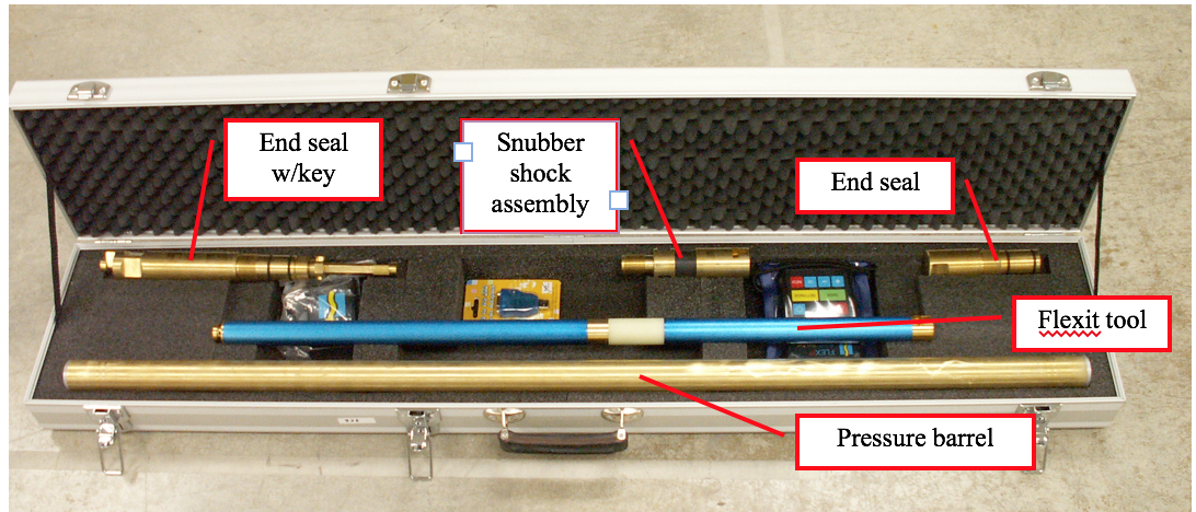
The FlexIT tool and brass pressure case kit.
Software Installation
If you are installing the software on a new computer, you must register the tools after installing the FlexIT software, version 3.5 (setup.exe file on TAS>dml>software>labsystems>Flexit). You will see an error message during opening communications if you start a survey without registering the tool.
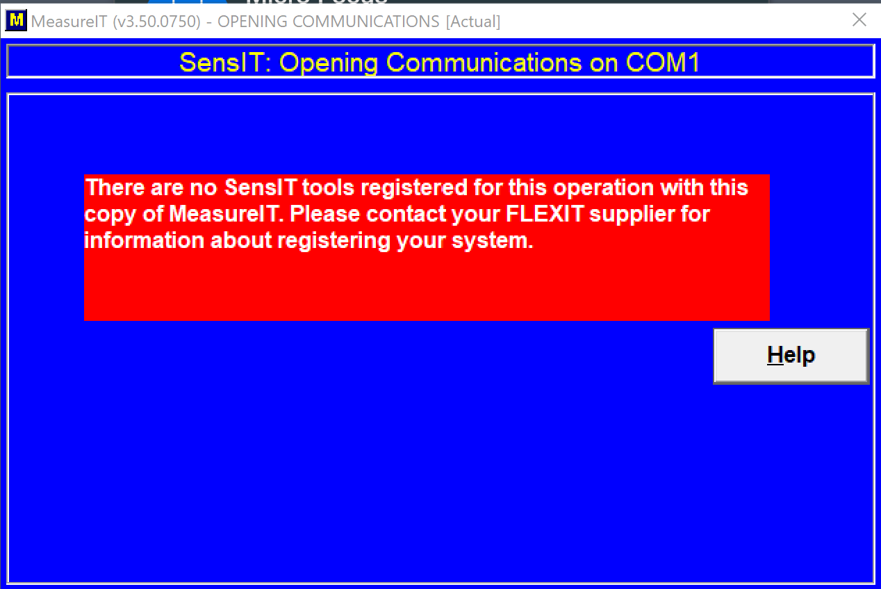
Error message if a tool is not registered
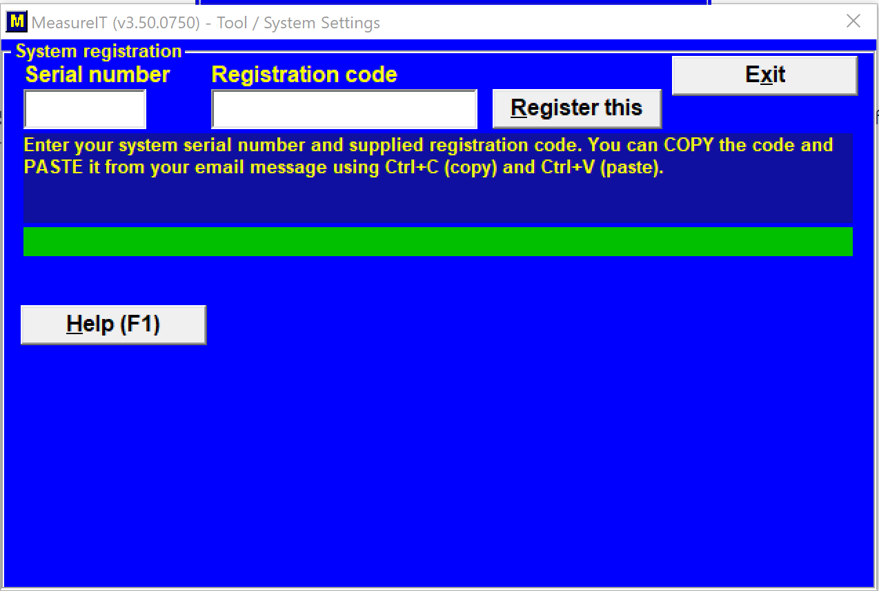
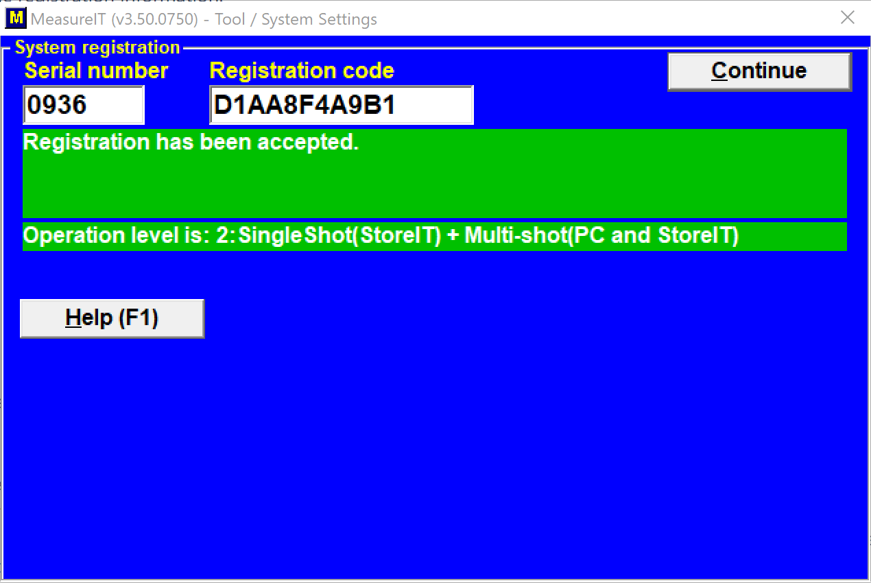
To register a tool, open MeasureIT 3.5 software. Click the Set-Up button, then click the Tool Set-up and Register SmartTool buttons respectively. Type in the serial number and registration codes for each tool one at a time and then click Register This.
The tool(s) will then be available for you to select when setting up for a run. Ignore any screens about sending off the registration information.
FlexIT tool registration |
Confirmation of registration |
|---|
IODP FlexIT Tool Information
s/n | Reg. number |
|---|---|
0936 | D1AA8F4A9B1 |
0937 | 9A952918021 |
Tool Setup
After arriving on site the technician will edit the default survey data to reflect the proper geomagnetic values for the area:
- Get the latitude and longitude of the location from the Bridge or from the Daily Operations Report (DOR) sent by the JR Operations Superintendent, and go to the website NCEI Geomagnetic Calculators where a calculator will provide the proper geomagnetic values. If the Internet is not available, please see Appendix 1. To convert latitude and longitude in the format used by the NCEI/NOAA, use the website Latitude / Longitude Conversion.
- Open MeasureIT, press Set-up (Figure 1) and then Default Survey Data (Figure 2) buttons to edit the Magnetic Field and Dip values for the magnetic Integrity Check (MagIC) and enter the default survey data.
- Use the slider down on the left hand side to access the other portions of the window (Figure 3). Hit Apply when the default information has been set when finished to return to the main menu.
- Default Survey Data is also where measurement units and intervals are set.
- Use The Tool Setup button (Figure 2) to set your default file location for surveys as well as enable Time-Based Continuous Survey (TBCS) mode (Figure 4).
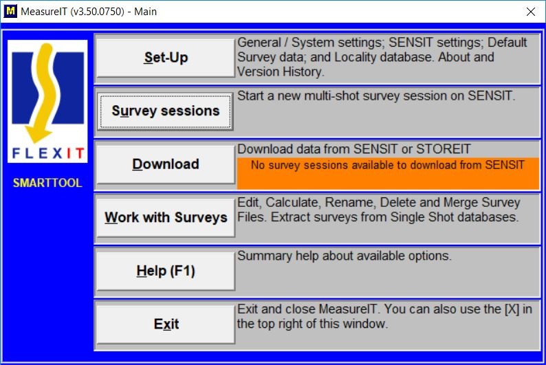
Figure 1
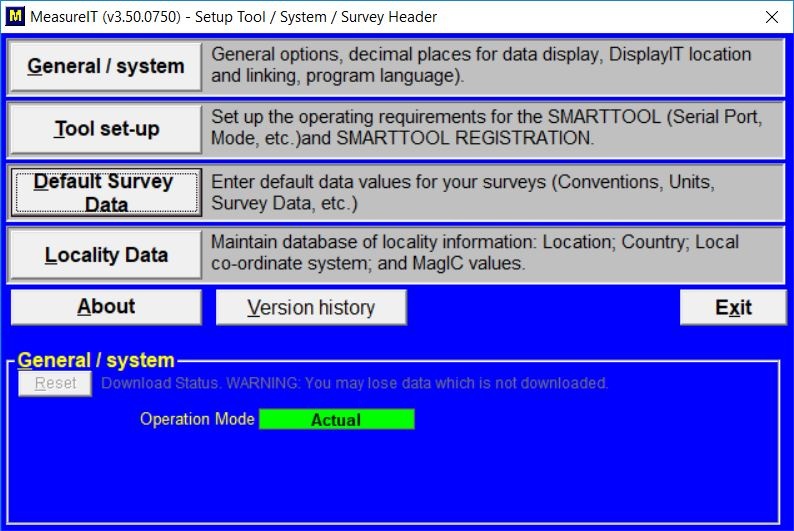
Figure 2
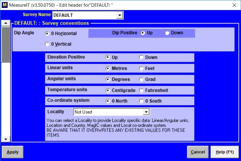
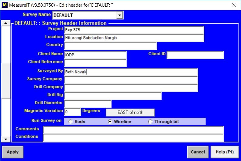
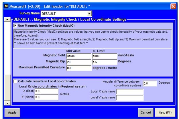
Figure 3 Default Survey Data screens. The left most window displays the proper default survey settings including units, the middle screen is where a user will enter the expedition, location, and other header information, and the right most window is where a user will enter the MagIC settings. Note that these different windows are accessed by sliding the bar on the left side of the screen in MeasureIT.
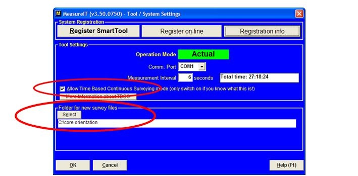
Figure 4 Specifying file location for your surveys and enabling time based continuous survey mode.
Starting a Survey
1. Have your unjacketed tool with batteries installed within a 5-10 meter line of sight to the TransIT PC adapter attached to the computer’s serial port.
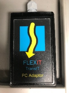 TransIT PC Adaptor
2. From the MeasureIT main menu (Figure 1), press the Survey Sessions button. Select your tool’s serial number (printed on the tool casing) from the list and hit Continue (Figure 5).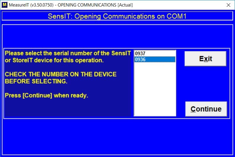
Figure 5 Communications initialization window
3. Verify that the tool is talking by clicking Measure Angles. (Most likely the data will make little sense inside the ship because of all the steel but the tool should be at least measuring and reporting.) Move the tool around and ensure that Measure Angles reports the changes. If not, make sure you are linking with the right tool! Our tools are stored close to each other and may also link if selected incorrectly, depending on your location.
4. Click the radio button for Time-based continuous survey as indicated in Figure 6. Select Continue/Initialize tool when finished.
a. Note that at a minimum 6 seconds between shots you have about 27 hours to acquire data before the memory fills up. Our tools have been run as long as 25 hours without incident, but it may be advisable to pull them every 8-12 hours to avoid too much data loss in case of problems.
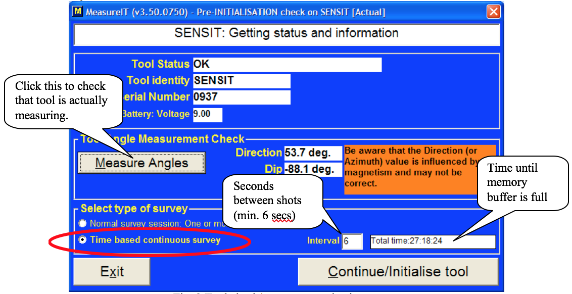
Figure 6 Tool check/survey type selection screen
5. You will be presented with a window telling you that it’s time to start your synchronization file for depths. We do not have to create this file just yet; it will be used during the processing phase though.
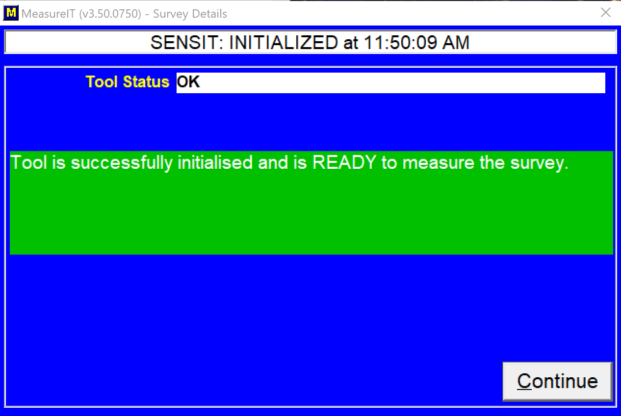
6. Additional windows appear with status information about tool initialization; hit Continue if everything is okay.
7. Give the survey a name, such as “{Site}-{Hole}-{start core}-{end core}” or similar (Figure 7). Verify that the measurement units are correct. The other fields should be ignored. Hit Continue when finished.
a. Note that “the clock is ticking” so avoid starting a survey hours before handing the tool to the Core Techs (CT’s).
b. Once the survey has started, the window will appear as in Figure 8.
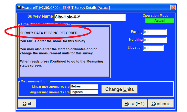
Figure 7 Survey naming and unit selection screen
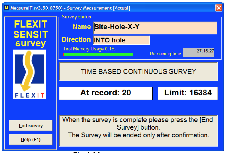
Figure 8 Real-time measurement status screen
8. The tool is now ready to go. Place it in its brass pressure case, snug up the end pieces and turn it over to the Core Tech (Figure 9A-B).
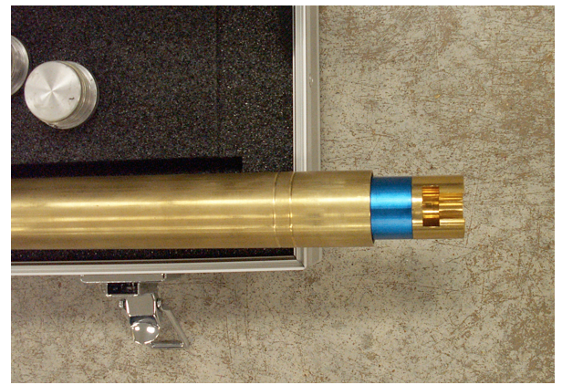
Figure 9A: Insert the tool into the pressure case’s open end as shown (keyway out)
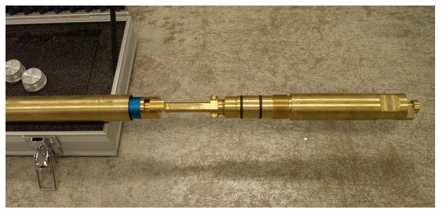
Figure 9B: slide the key end of the other end seal onto the Flexit tool, insert it into the barrel and tighten. Hand the assembly to the Core Tech for final rigging with the snubber shock and IODP pressure case.
9. Keep track of the times that the tool is on bottom. Stand pipe pressure data and the time on deck for each core can be used to determine when the tool was on bottom. Standpipe pressure peaks just before the core barrel is fired into the sediment, so the orientation period is ~5 minutes before the peak. Please see an ET or Ops Supervisor for a demonstration on accessing the standpipe pressure data.
Data Retrieval and Processing
This version of the software can only do one thing at a time when performing continuous surveys, so you won’t be able to configure another tool on the same computer while the first tool is still waiting to have its survey ended. Therefore, if orientation continues and you need a second tool to give to the CT’s then it will have to be configured on a different computer that is also running the Flexit software and has a TransIT transceiver attached. Then it can be measuring while you download the data on the first tool from the starting computer. We have a site license for the software, so it can be installed on as many PC’s as necessary, but only three TransIT radio-sync devices exist (as of August 2022, one is connected to the KAPPA PC in the pmag lab, one to the PC in the downhole lab, and one is spare and kept in the Orientation Tool drawer in the downhole lab).
We have found through experience that it is preferable to download all of the survey data from the tool, process it, and then put it into a spreadsheet instead of pre-selecting exact data windows based on the driller’s worksheet. That allows the user to look at the entire data set and not potentially miss anything by assuming the orientation data window is exactly the same as a given time on bottom (TOB) from the driller. Sometimes the actual orientation windows may be a minute or more different than the time listed by the driller due to factors such as typos or core barrel rotation late in the orientation period.
- After receiving the tool from the CT’s, unload the tool from its brass pressure case and keep it within a 5 meter line-of-sight of the TransIT adapter to the computer. Return to the measurement screen (Figure 8) and click End Survey. An option to download the data follows.
- A confirmation screen appears to make sure you really want to finish the survey (Figure 10). Select End Survey Session.
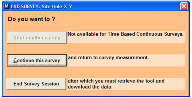
Figure 10 End survey confirmation screen
3. Click Start Download to begin the data download (Figure 11). You’ll need to select your tool from the list as before. Click Continue.
a. It takes about a half-second per shot for the data to download, e.g. an 8-hour survey at 6 sec/shot should take around 40 minutes to download. The downloading survey window will be displayed throughout the download process (Figure 12).
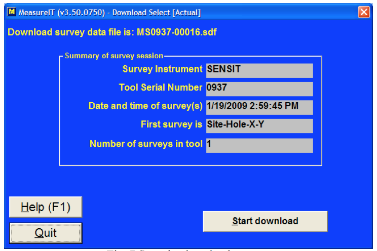
Figure 11 Start the download process
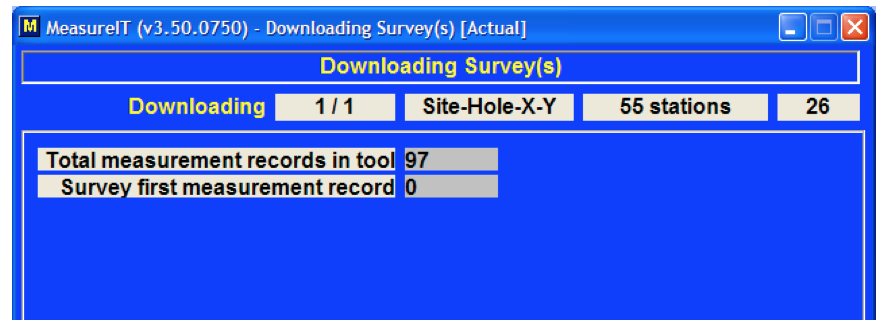
Figure 12 Download-in-progress screen
4. After downloading the data processing screen appears (Figure 13). This is where you will select the synchronization file.
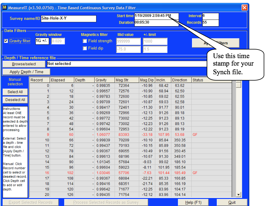
Figure 13 Preliminary downloaded data screen
5. Select Browse/select under the Depth/Time reference file heading and navigate to the mega_sync.txt file. This file is usually found on the C drive in a folder called Core Orientation. Click OK. If the megasync file does not already exist, refer to Appendix 5 for instructions on creating a new megasync file.
6. Click Apply Depth/Time.
7. Scroll down the data window. You will see your windows of interest highlighted in green. Any suspect data that fails the non-optional Gravity check (1G +/- 2%) will be flagged in lighter green with red text.
8. Click the Process Selected Records as Survey (Figure 13). A file named {your survey name}_FLT.svy is created. This will calculate the values for Magnetic Tool Face (MTF), the primary information IODP uses to orient cores, as well as a variety of other data.
9. Proceed to the Multishot Calculation Stage 1 screen (Figure 14). Click the ‘Do not review’ button to skip the data review screens. They are of limited use to us because we are not performing a “traditional” downhole survey..
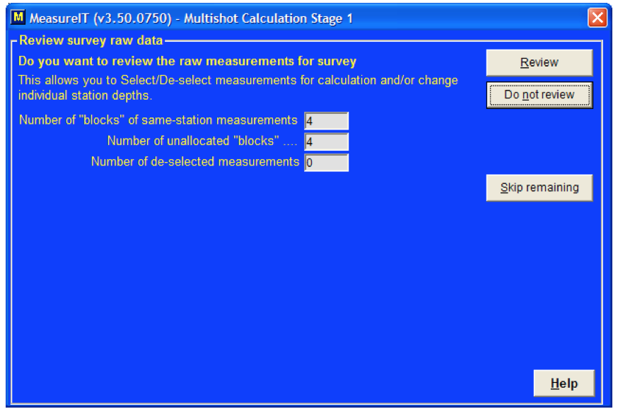
Figure 14 Stage 1 calculation options screen
10. The final screen will reveal the results of the survey (Figure 15). You can review both the raw and processed survey files by navigating to the file location you specified as shown in Fig. 1B. All files are in ASCII text despite the file type suffix (.rsy=raw survey, .svy=data-reduction results, .csy=continuous survey, .dtf=depth/time file). Select Continue.
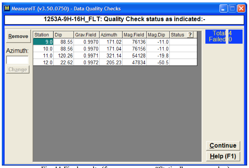
Figure 15 Final results (for our purposes, “Station” = measurement every 6 seconds)
11. The next step is to calculate out the number of the first station that should be very close to the orientation window for each core (Figure 16). Consider that station numbers in a survey file are time proxies, i.e. each station represents 6 seconds. You can get the tool initialization time and date from either the raw or processed survey file (in GMT since IODP workstations are set to that zone). It may be easier to convert the time to local ship’s time for the processing step and to recollect the timing of some operational details that may pertain to the orientation data.
Example: tool start time (from the raw survey file) was 5:25 am local or 0525 hours. According to the standpipe pressure data and time on deck, the tool was on bottom and orienting at 0737 hours for core 3H, 0853 hours for core 4H, and 1012 hours for core 5H. The time difference from tool initialization to core 3H is 132 minutes. Multiply by 10 shots/minute since our tools measure every 6 seconds and you get 1320 measurements taken before you should see your orientation window begin. Similarly, there is 76 minutes between time-on-bottom (TOB) for core 3H and 4H, so add 760 to core 3H’s starting point of 1320. Your window for core 4H should start around station #2080. Finally, core 5H’s window will be around station #2870 since there were 79 minutes or 790 shots between core 4H and 5H.
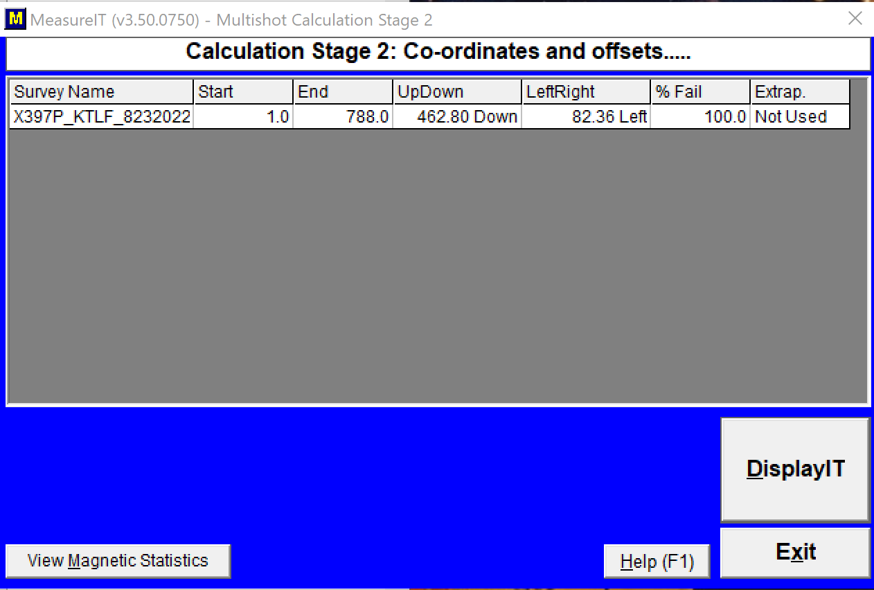
Figure 16 Calculation of station numbers
If you wish to see the data in DisplayIT application, click DisplayIT, then Yes at the pop-up window to see the data (Figure 17). Click Exit otherwise.
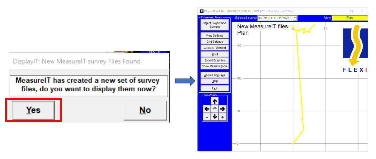
Figure 17 Displaying the data in DisplayIT software
12. Copy the data portion of the processed survey file (*_FLT.svy) into Excel and parse it. Hide or delete columns of no interest such as Easting, Northing, Elevation, UpDown, LeftRight, Shortfall, ToolRoll, and DLS.
Optional - for ease of scanning apply conditional formatting to the Temperature, Magnetic Field and Gravitational Field columns: change cell’s color if temperature is below 3° C (your bottom hole temperatures may be higher), Mag. Field is less than 50000 nT (check field model for your location and add a ‘fudge-factor’ for the drillstring) and Gravity is less than .980 or greater than 1.02. Scroll down the processed survey file to the station numbers you calculated in step 10. You should see very repeatable data particularly in the MTF, temperature, and magnetic dip fields. Suspect gravitational field measurements will have changed color from conditional formatting making them easy to delete from the total records to be averaged. Average your ‘clean’ records and provide the MTF value to the paleomagnetists. Consider keeping a table with other statistics such as the standard deviation, number of readings averaged, and approximate time spent orienting for each core .
This Excel spreadsheet should contain all data of interest from the survey and optionally plots of orientation data as a function of time.
Uploading Data to LIMS with MUT2
Uploading orientation data to LIMS requires a few steps done by the pmag technician:
- Calculating core orientation statistics and plotting data in an Excel spreadsheet
- Creating a .csv file which will be read by MUT2
- Gathering the needed MeasureIT files
- Copying the files in a specific folder for MUT2
Creating the .csv file
To upload orientation data to LIMS, the pmag technician must create a .csv file with Excel, in the same way as for the Icefield orientation tools. This .csv file is the file that MUT2 reads to upload the data to LIMS.
The averaged core orientation statistics for each core must follow a specific format or MUT2 will not recognize or upload the files to LIMS:
- Spelling must match the example column headers in Figure 18
- Format the different entries with adequate significant digits. For instance, Azimuth and Magnetic Tool Face columns to have two significant digits.
Save the file as .csv with a name that includes expedition number, site, hole and first core contained in the .csv file (i.e., Exp354_U1451A1H.csv)
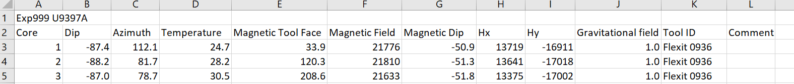 Figure 18. Required header formatting for core orientation data
Here is a template file with the exact headers in CSV format:
There should now be four files with identical file names and the extensions on the files should be .csv,.csy, .svy and .xlsx.
Open MegaUploadaTron 2 
The four datafiles should appear with "Orientation Datafiles" as Analysis (Figure 19).
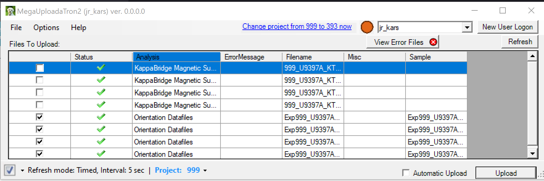
Figure 19. Orientation datafiles in MUT2 ready for upload
Click "Upload". If the upload is successful, the four files will be transferred to the archive folder at C:\Core Orientation\Data\archive.
The orientation data can be found in LORE in Magnetism>Orientation (ORIENT)
Troubleshooting Uploads
Symptom | Solution |
Purple question mark in MUT2 |
|
File appears to upload (moves to archive file), but does not appear in LORE | Check the formatting within the .csv file, especially the significant digits of values (LORE has a maximum limit of digits). |
An error message appears saying that a line in the file does not have the correct number of columns | Check that there is no comma in the table, especially in the comment box. Comma is used as separator for the upload. LIMS reads the .csv file. |
Files will not upload and MUT2 hangs | Verify the the .csv file does not contain any extra empty rows of commas. If it does, delete them in a basic text editor, save, and retry. |
Tool Maintenance and Storage
- Clean and dry the tool after use, including the pressure case.
- Store tool inside the pressure case.
- Check the O-rings. Keep them clean, undamaged, and lightly lubricated. Use small amounts of silicon lubricant (Dow Corning 111). The O-rings seal the tool from invasion of drill fluid so it is important to make sure to check them regularly.
- Tighten the sealed Pressure Barrel threads by hand (never use a pipe wrench on the barrel).
- Avoid rapid tool acceleration, fast braking, drill string rotation, or impacts.
- Check for burrs on the tool end cap and lightly sand them off if they are found. Burrs may damage the inside of the pressure barrel.
Appendix
Appendix 1: Using the offline geomagnetic field calculator software
This calculator uses a model for the geomagnetic field from 1900 to 2010. It will not allow you to enter a date after 2010.
1) Copy the software from TAS/Software/labsystems/Flexit/geomagnetic field calculator/Geomag61_windows folder to your local PC.
2) Double-click the Geomag.exe program in your new folder.
3) Follow the onscreen prompts. Enter IGRF10.cof for your model, although either model should give similar results for our purposes.
4) Choose option 2, month, year and day for the date entry.
5) Choose 1, single date for the range option.
6) Enter the year, month and day as requested.
7) Select option 1, Geodetic coordinates.
8) Select option 2, meter units.
9) The geodetic altitude above mean sea level (AMSL) is zero, of course!
10) Select whichever mode of latitude/longitude notation you prefer, then enter your coordinates. Winfrog or the bridge is a good place to locate this information.
11) The results are then calculated. For our tool configuration purposes you should make a note of F (total field in nanoTesla; you can safely round to the nearest 500) and Dip. You might also make a note of the individual magnetic field vectors X, Y and Z for occasional comparison with the raw data from the tool.
12) Follow the onscreen prompts to quit or calculate more values.
Appendix 2: Guidelines for “suspicious” tool readings
- Tool motion indications: According to Flexit, a reading is considered suspect if it exceeds ±2% of 1 gravity.
- Absurdly high or low magnetic field readings: readings more than 20000 nT above the values for the location (derived in Appendix 1) may indicate that the tool is either faulty or may not be centered in the non-magnetic collar. Low values are probably from faulty magnetometers inside the tool. Keep in mind that magnetic field and dip will be considerably higher than normal for your location due to the presence of the drillstring, but you can still obtain usable orientations.
- Excessive variation of calculated results within a time window for orientation:
- Manually scan the file above and below the supposed time period for more consistent results. The time window you were given may be incorrect (typos/transcription errors in the times). Conditional formatting in Excel is a good way to quickly narrow down possible orientation windows.
- Tool rotated during orientation period. You may be able to find more stable data at the very end of the orientation window. Use the latest stable data for that core.
- Low battery voltages may cause bad measurements.
- We have occasionally seen “rifling” when apparently good tool results do not apply correctly to all or some sections of the recovered core. This can happen if the tool is stationary and got good results, but the actual core twisted inside the barrel when it fired into the sediment. Remember, orientation is performed before the core is shot, not afterwards.
Appendix 3: Disabling the tools in case of explosives work on the rig floor
If there is any question or concern that the radio-frequency transmissions (433MHz, one of two internationally-permitted frequencies for short range radio control) involved with configuring or downloading the Flexit tools may pose a risk to the rigging of explosives for blowing pipe, then do the following:
- Keep the Flexit tools inside their brass pressure cases with the aluminum end caps installed. This should block any communication with the tools from the computer. For absolute certainty, remove the tools’ batteries as well. (TO CHECK: does battery-removal blow the memory buffer of survey data??)
- Remove the TransIT PC adapter from the computer’s serial or USB port and remove its 9V battery. Be sure you get all Flexit-enabled computers with adapters, there may be up to three of them.
Appendix 4: Flexit file types, locations and extensions
There are a number of files associated with a given survey. Some files are only created after you process the raw survey using the synchronization file. Others are simply log files that you can read for information. Still others are artifacts of a known bug in the software† and will cause trouble unless they are deleted after download.
File Type | extension | Normal location |
TBCS raw survey file as downloaded from tool (magnetometer and accelerometer raw data, battery voltage, tool temperature) | *.csy | Your default file location in the Flexit software (Fig. 1b) |
TBCS synchronized raw survey file | *_FLT.rsy | Created post-processing at the same location as your raw .CSY file |
TBCS synchronized processed survey file | *_FLT.svy | Created post-processing at the same location as your raw .CSY file |
Sync file location pointer | *.dtf | Created post-processing at the same location as your raw .CSY file |
†temporary survey data file (created when starting a download) | *.sdf | C:\Documents and Settings\All Users\Application Data\Flexit\MeasureIT |
Survey synchronization file | *.txt | User-selectable location |
MeasureIT.ini (initialization file for Flexit software) | *.ini | C:\ Documents and Settings\All Users\Application Data\Flexit\MeasureIT |
Measureit_LOG (verbose logs of tool downloads and other user/software interactions) | *.txt | C:\ Documents and Settings\All Users\Application Data\Flexit\MeasureIT (see also .\Logfile Archive for date- and time-stamped older log files) |
† Important note: be sure to delete or rename the file extension of this file after downloading a survey to the computer. If you do not do this and send the same tool down for another survey, the next download will contain a copy of the previous survey’s data, not your current survey. This is a bug in the current MeasureIT software version. You must delete the .sdf file.
Appendix 5: creating the “Mega-Sync” file
a) Start a new workbook in Excel.
b) You will be filling 2 columns with numbers. The first column is time in seconds per station (our default is 6) and the second column will be station number starting with 0.
c) Increment all subsequent columns: add 6 to the first column and 1 to the second column in the following fashion down to row 16383:
6 | 0 |
12 | 1 |
18 | 2 |
24 | 3 |
30 | 4 |
36 | 5 |
42 | 6 |
48 | 7 |
54 | 8 |
60 | 9 |
66 | 10 |
72 | 11 |
... | … |
d) Use the concatenate function in Excel to group the 2 columns together delimited by a semi-colon.
e) Open another workbook. The first row must contain “SynchTime=MM/DD/2009 HH:mm:ss” with no quotation marks.
f) Paste-special (values only) the concatenated data column in your first workbook.
g) Save the file as Text. It is now ready to use as a synchronization file of any size you need for your survey.
Appendix 6: Battery Life Considerations
There are two batteries of concern when running surveys: the actual tool battery itself and the battery inside the TransIT transceiver. Both battery voltages must be monitored to avoid losing survey data.
The tool battery consists of three CR123 lithium camera batteries attached together and encased in heat-shrink tubing with a small wire harness and 2-prong connector. Battery voltage from the pack can be 9.5V or better if the individual batteries are very fresh. The battery in the transceiver is a standard 9V alkaline cell.
Extensive bench testing demonstrates that the tool batteries will last for a very long time (Figure 20) , but experience has shown that it’s advisable to change the battery when the voltage during a survey reads approximately 8.5 volts. The tool battery resting voltage is displayed when you first set up a survey (Figure 6). However, a more accurate assessment of the tool voltages are found in the raw survey file (*.csy file). That file will give the user a much better idea of the actual state of the battery when in use downhole. Scan the raw file after each survey or plot voltage vs. station number (i.e. time) during data reduction.
As a standard operating procedure each TransIT battery should be changed at the beginning of every cruise that will be performing core orientation. If the battery fails during download, the download itself will slow down immensely and you will lose all survey data past the point where the TransIT battery had insufficient voltage (zeros will be written to the data file).
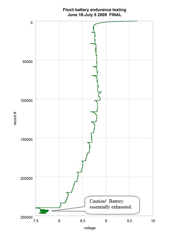
Figure 20 Flexit new-battery voltage decay at room temperature from repeatedly running ~24-hour surveys followed by downloading the tool’s data. Deflections in the curve represent the data download periods. The vertical axis translates to over 410 hours of survey time (one record = 6 seconds). See raw survey files (.CSY) for voltage information during actual surveying.
LIMS Component Table
To avoid duplication, please see the LIMS Component Table under the Icefield MI-5 Orientation tool user guide.
Archived Versions:
- FlexitOrientationTool_UserGuide_X397T_SEP2022
- FlexitOrientationToolUserGuide_exp378.pdf: PDF version of this wiki page as of 2020-02-24