Table of Contents
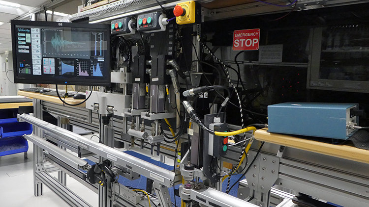
The P-wave Velocity station.
I. Introduction
The P-wave velocity gantry measures the speed at which ultrasonic sound waves pass through materials that are placed between its transducers. The three orthogonal sets of piezoelectric transducers allow the velocity to be determined in the X-, Y-, and Z-directions (Figure 1) on working-half split-core sections. The P-wave bayonets (PWBs) measure the velocity along the core (Z-direction) and across the split-core face (Y-direction), and a P-wave caliper (PWC) measures the velocity perpendicular to the split-core face (X-direction). A laser measures the position of the top of the split-core section and calculates the position at which the velocity was measured (this is recorded as Offset in the LIMS Database). For discrete sample cubes, the velocity is measured along each of the three axes separately using the PWC. Mini-cores are measured along the axis of the cylinder (X-direction) using the PWC. For discrete samples cubes and mini-cores, all sample information, including offset, is entered by the user when the sample was taken.
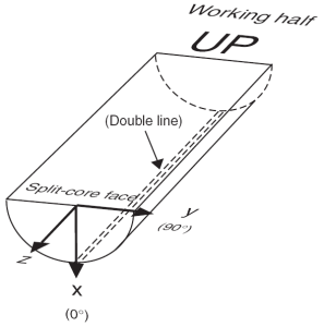
Figure 1. Section half measurement directions.
Method Theory
Measurement of P-wave velocity requires an estimate of the travel time and an accurate measurement of the ultrasonic P-wave path length through the sample.
Velocity is defined as follows:
velocity = pathlength/traveltime, or
v = dS/dt.
Traveltime measurement is estimated by an algorithm for graphical first arrival pick. An ultrasonic pulser generates a high-impulse voltage, which is applied to the ultrasonic transmitter and thereby induces oscillation of the crystal element within the transducer-specific frequency band. A trigger pulse from the pulser is then applied to the oscilloscope to record the waveform from the receiving transducer.
By measuring the acoustic traveltime of the waveform through a standard of known pathlength and velocity, the difference in expected travel time and actual travel time provides the instrumentation-specific time delay. Subtraction of the system delay time (+ liner material propagation time, if required) from the total traveltime gives the traveltime for the ultrasonic pulse through the sample.
Precise thickness of the sample, or path length, is derived from the readout of an Acuity AR700 laser displacement sensor. The laser offset correction is determined during the calibration process and requires that the system fully close the transducer caliper when the software is opened and activated. Therefore, do not place a core section underneath the transducers when the software is started.
The chisel (bayonet) transducers are fixed at 82.32 mm for the z-axis (downhole) and 31.70 mm for the y-axis (see figure 1). As mentioned above, the x-axis caliper separation is derived from an Acuity AR700 laser.
Traveltimes for samples are calculated as follows:
x-axis = total traveltime – x-system delay time – liner traveltime (section-halves only)
y-axis = total traveltime – y-system delay time
z-axis = total traveltime – z-system delay time
Liner traveltime is calculated as the liner thickness (typically 2.7 mm) divided by the published liner material velocity (cellulose butyrate = 2140 m/s).- Wasn't this experimentally determined?- Currently we are using 2100m/s.
T he travel times for any measurement signal is based on either a user selected location on a graphical display of the first arrival wave (manual pick), or a software auto-pick feature, which attempts to determine the first arrival of the measurement signal. The auto-pick feature will search for the first instance of a signal stronger than a user set threshold value (milli-amps). Next it will take the absolute value of the signal and determine where the wave-form crosses the graph's x-axis the 2nd time. It will then subtract an assumed 1/2 of wave length, and display the pick location on the same graphical display. This should get the travel-time of the measurement signal. Verification of the signal and pick location by the user is critical.
II. Procedures
A. Preparing the Instrument
- Double-click the MUT icon on the desktop (Figure 1a) and login using ship credentials. For more information on data uploading see the "Uploading Data to LIMS" section below.
- Double-click the IMS icon (Figure 1b). IMS initializes the instrument. Once initialized, the logger is ready to measure the first section.
![]() Figure 1. (a) MUT Icon. (b) IMS Icon.
Figure 1. (a) MUT Icon. (b) IMS Icon.
At launch, IMS begins an initialization process:
- Testing instrument communications
- Reloading configuration values
- Homing the caliper and bayonets. IMP: DO NOT place samples on the track before launching the software.
After successful initialization, the IMS Control and Instruments' windows appear (Figure 2).
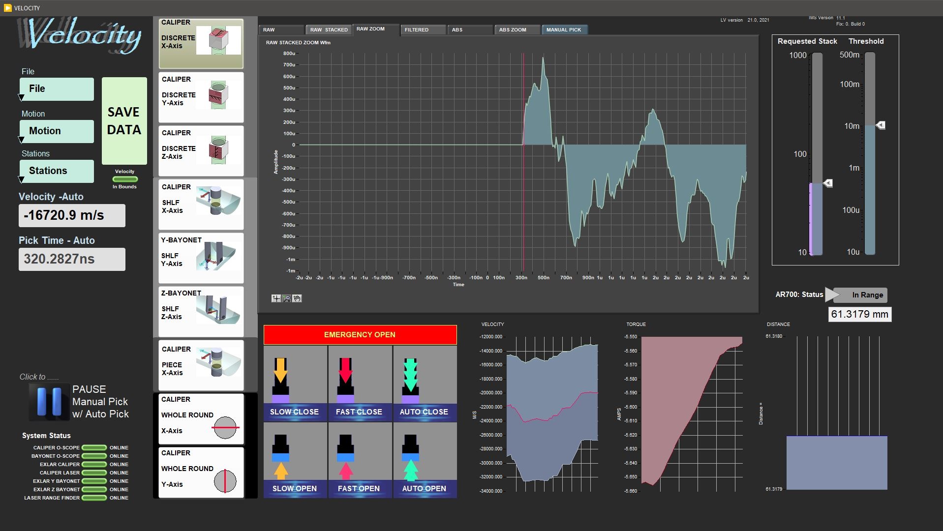
Figure 2. Main Velocity window.
***CAUTION: Make sure there are no samples or body parts underneath any of the sensors when starting IMS***
When first opening the program, all 3 sensors will go through a communication initiation process where they will move down and up. The program will display a warning message (Figure 3a) but will not stop the movement if nothing is detected on the rail. If an object is detected a warning window will pop up (Figure 3b).
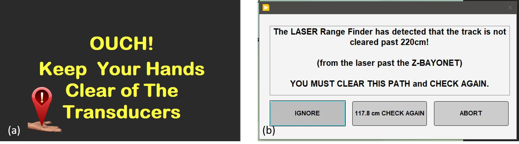
Figure 3. (a) Reminder message while opening IMS. (b) Warning message if an object is detected.
The software home screen allows the user to modify a number of setup and acquisition parameters directly, as well as control the motion of the transducers.
The main window (Figure 4) includes:
- Sample type and Measurement Axis selection: The user selects the type of sample, while simultaneously selecting the measurement axis via the pictured tiles, the current selection will be highlighted.
- Graphical Display Tabs: The RAW, RAW STACKED, RAW ZOOM tabs will display the measurement signal without mathematical manipulation. They also display the MANUAL PICK location as a vertical pink line. The ABS and ABS ZOOM tabs display the absolute value and the uncorrected auto-pick location, which should be
between the 1st and 2nd hump. These displays are crucial for evaluating the signal quality and pick locations. - Requested Stack and Threshold sliders:
- Requested Stack: The number of measurement signals the software will add together with the intent of increasing the signal to noise ratio. Each time it is adjusted a new set of signals will begin stacking. 100 stacks is a typical value.
- Threshold: Voltage level (y-axis of the graphical display mV) that the stacked signal must attain for consideration in a auto-pick. If the threshold is too low, signal noise may be selected as the first arrival. If the threshold is too high, the first arrival may be missed and included with the signal noise.
- Mini Graphs: VELOCITY graph displays the running average of the last 1,000 samples and the TORQUE graph display the torque applied by the actuators to the sample. The DISTANCE graph displays the AR700 distance readings.
- Motion Control Buttons: These control the up-down motion of the caliper and bayonets. The user may select to make slow, fast or automatic movements. EMERGENCY OPEN button will bring up bayonets and caliper simultaneously.
- Pause Button: By selecting the pause button, the user will be able to make manual picks and have the velocity of that pick displayed.
- Save Data: The save button is activated when an automatic velocity pick is within the velocity filter range or when a manual pick is made.
- IMS Control panel (Figure 5): Provides access to utilities/editors via drop-down menus.

Figure 4: Main Velocity Window with annotated sections.
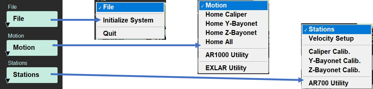
Figure 5. IMS Control Panel.
Before start measuring assure that the transducers are clean. If not, clean them with water and paper towels.
B. Instrument Calibration
The bayonets and caliper transducers must be calibrated and the system delay determined whenever a check standard is out of range, +/-2.0% of the expected velocity. There is a separate utility for each one:
- The bayonet transducers are calibrated by back-calculating the system delay from the total travel time, for the y- and z-axes, from the transducer separation value and theoretical velocity of distilled water at the temperature of the water bath.
- Calibration of the caliper requires the transducer and system delay to be calibrated concurrently. The transducer separation is measured with a displacement laser.
System delay is derived from the separation for the different calibration standards and travel time is derived from a travel time pick algorithm.
The calibration uses the derived velocity of the standard material to test for acceptance or rejection of the data. Aluminum and acrylic, materials used as calibration standards for the caliper, have a published sound speed of 6295 m/s and 2730 m/s, respectively.
Caliper Calibration
The Caliper Calibration Utility calibrates the laser offset and the delay of the system at the same time.
Measurements are taken at standards with the same velocity but with different heights. The operator can choose the number of standards used and the material. A linear correction is applied to calibrate the laser offset, while the system delay and velocity is calculated from the time measurements.
By convention a set of six acrylic standards with increasing sizes (15.07, 20.00, 30.03, 34.99, 34.90 and 45.01 mm) are used. They will be measured one by one, following next steps and the same procedure as an ordinary sample.
To open the Caliper Calibration Utility select: Stations > Caliper Calib. from the IMS panel menu (Figre 5). The Caliper Calibration window will open (Figure 6).
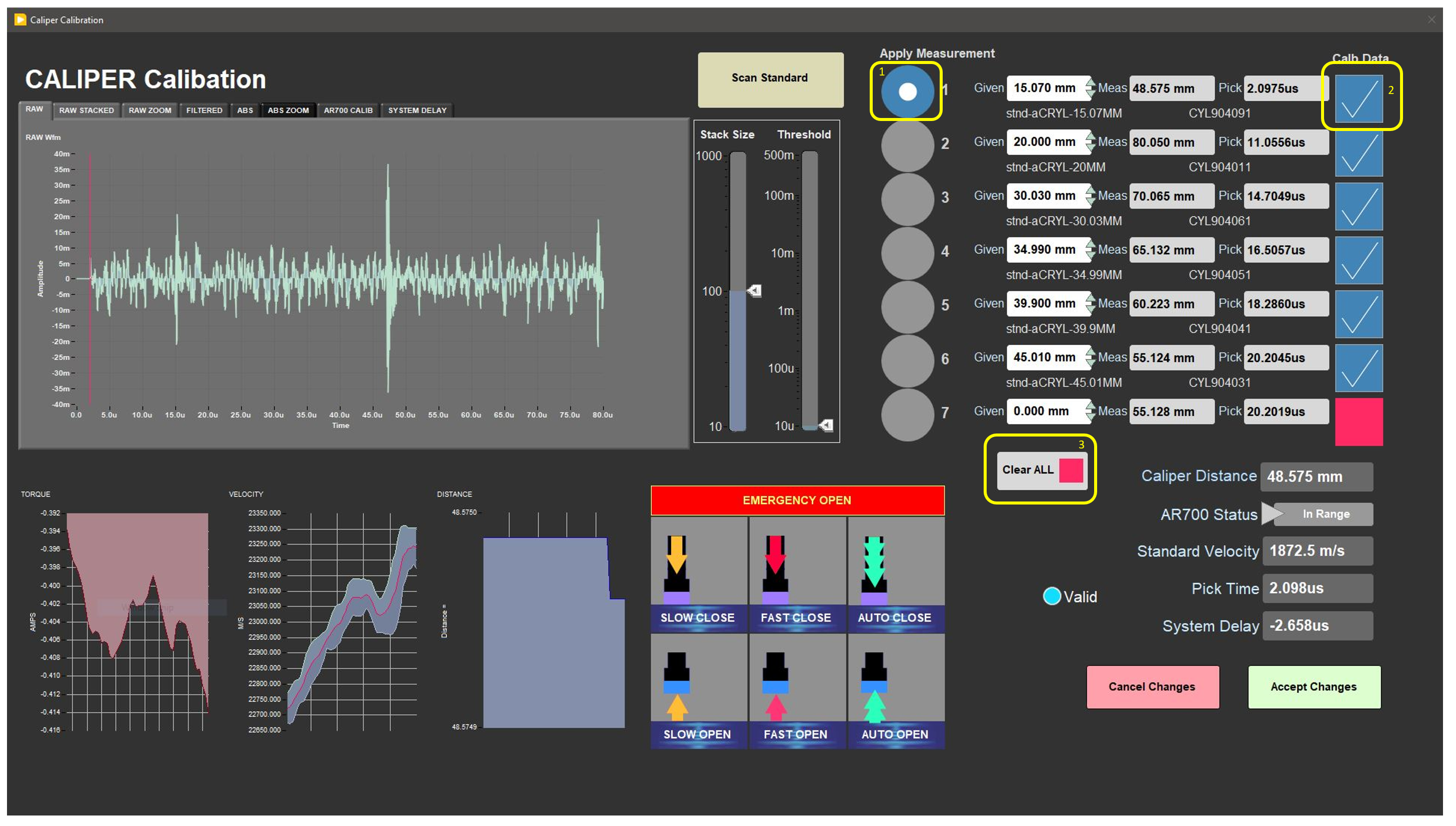
Figure 6. Caliper Calibration window.
In the Caliper Configuration window there are 7 row of calibration data which will auto populate from the previous calibration. You can standards by scanning in new id's and/or you can update the given thickness. Any changes will available in subsequent calibrations. If the row already has the correct ID and thickness you do need to re-scan the id.
In Figure 6 (item 1) there are 7 round buttons on the left side of each row. Only one can be selected at a time and the one selected will be updated constantly by values being measured. When you are satisfied you have the correct time pick, select the next standard to measure. The previous values are frozen while you measure the remaining samples. If you reselect that standard the values will be overwritten with the current measurement, so choose wisely.
The button on the right-hand side (Figure 6, item 2) are selected if you want to use that value in the calibration. Remember you need at least two for calibration but use all 6. Keep in mind that the program is always re-calculating the calibration values (Figure 9 and Figure 10) and it is ok to select and unselect value to see the affect on the calibration values. The same with remeasuring just make sure you apply the correct time pick to the correct sample.
Quick step by step
- Select the standard
- Optional only if needed
- Click Scan Standard
- Use bar code scanner and scan label
- Click OK
- Place the first standard in the caliper.
- Click AUTO CLOSE
- Set the threshold to pick the first arrival
- Set you stack to at least 100 and wait for the time pick to stabilize. Increase the stack as necessary.
- When satisfied select the next standard
- Click AUTO OPEN
- Repeat steps 2 through 8 for each standard.
- Select the standards to use in the calibration (can be done at anytime)
- Click Accept Changes or Cancel Changes
To clear the rows, de-select the rows you want to clear (right-hand Boolean controls) and then click Clear All
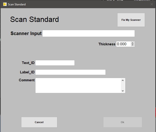
Figure 7. Scan Standard window.
How to verify first arrival pick:
Verify the software is picking the first arrival wave in the Raw Stacked graph tab. You can adjust the threshold scale bar to achieve the proper pick location (Figure 8). Observe the graph to verify the system is getting a clean signal. If you are not getting a clean signal, follow the steps in the trouble shooting section of this guide. Also, verify the auto-pick location in the Absolute Value tab (ABS or ABS Zoom). This pick should be at the zero crossing after the first significant wave form above noise (Figure 8).
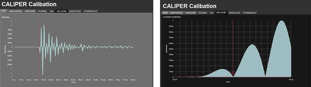
Figure 8. Caliper Calibration Window:. Raw data graph tab (left) and the ABS zoom graph tab (right).
Before you Accept
Check the standard's calculated velocity (= inverse of the slope) it should match the known material velocity as follows:
- Acrylic velocity= 2730 m/s ± 2.0 %
- Aluminum velocity= 6295 m/s ± 2.0 %).
To calculate the laser offset, the zero contact position offset was determined for the transducer and a small slope correction values (Figure 9).
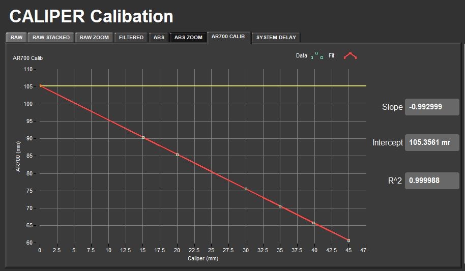
Figure 9. Laser (AR700) offset calculation.
To calculate material velocity and the system delay value the pick time is measured during the calibration (Figure 10).
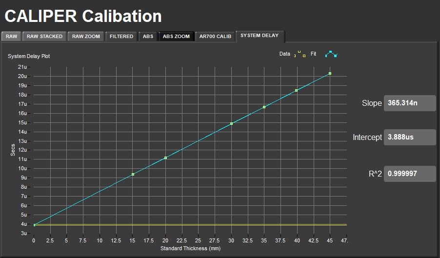
Figure 10. System Delay regression line.
Bayonet Calibration
Because the distance between the bayonets is fixed, only the system time delay needs to be calculated. This is achieved by measuring the velocity in water of known temperature, the difference between the known and measured value is due to system delay.
To open the Bayonet calibration window (Figure 12), select Stations > Y-Bayonet Calib. or Z-Bayonet Calib. from the IMS panel menu (Figure 5).
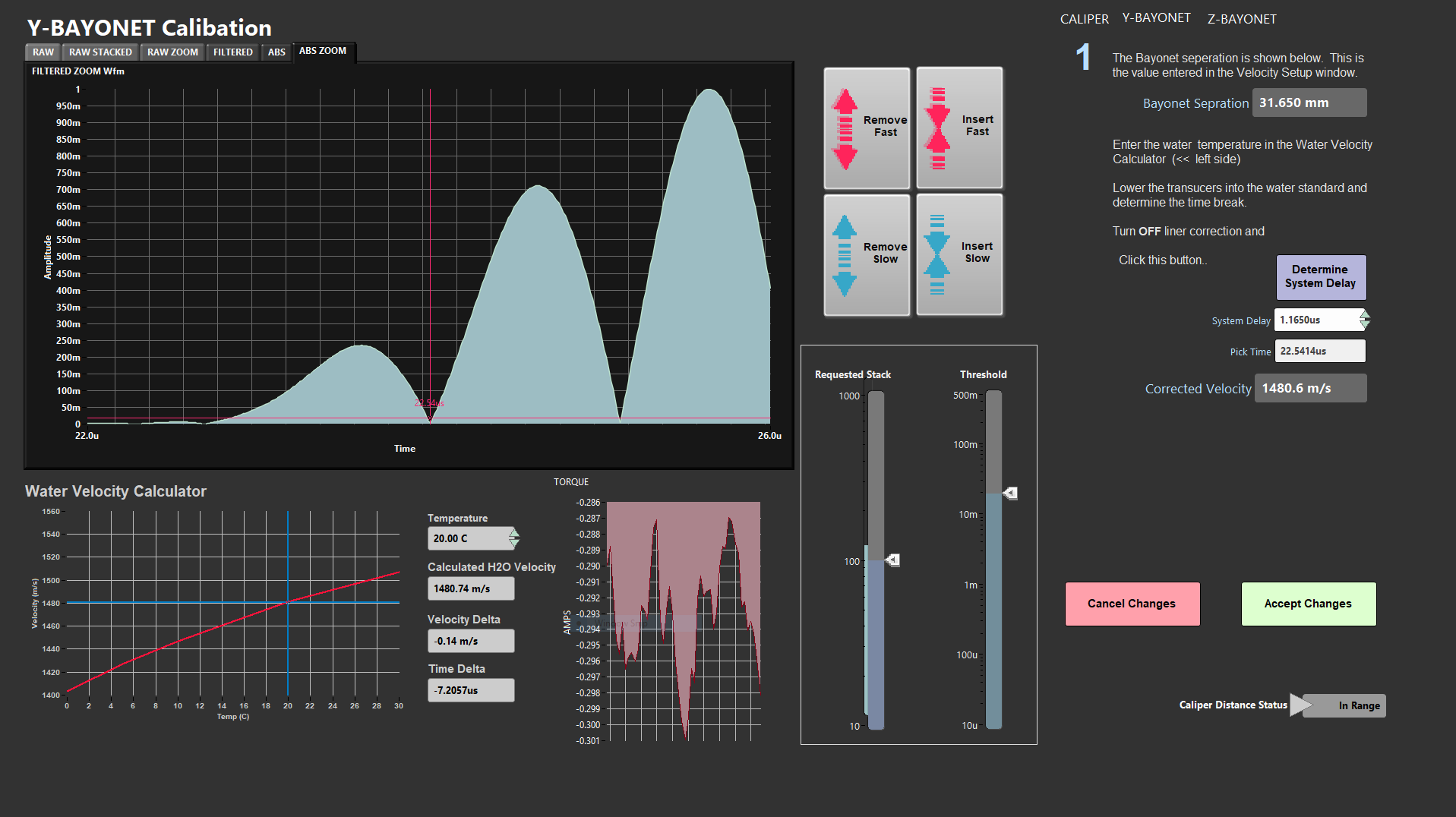
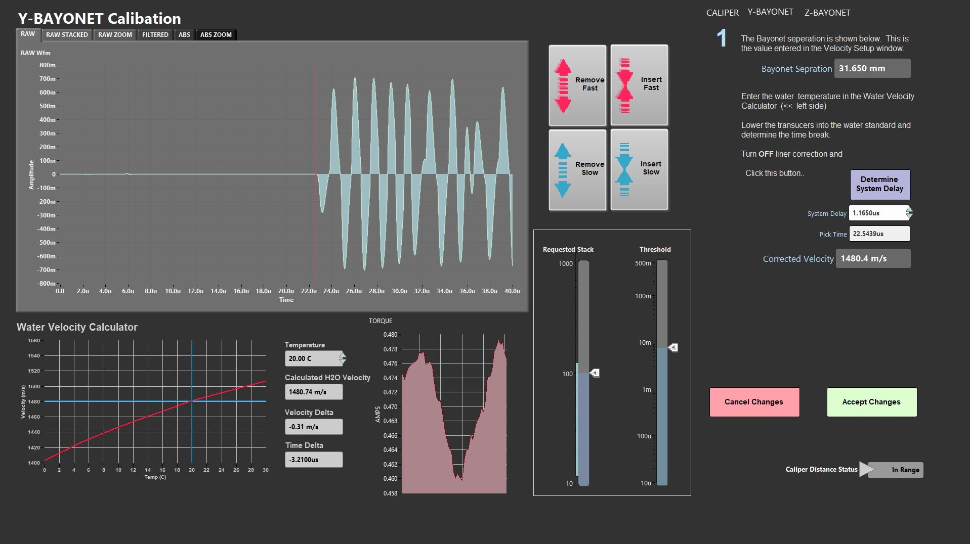
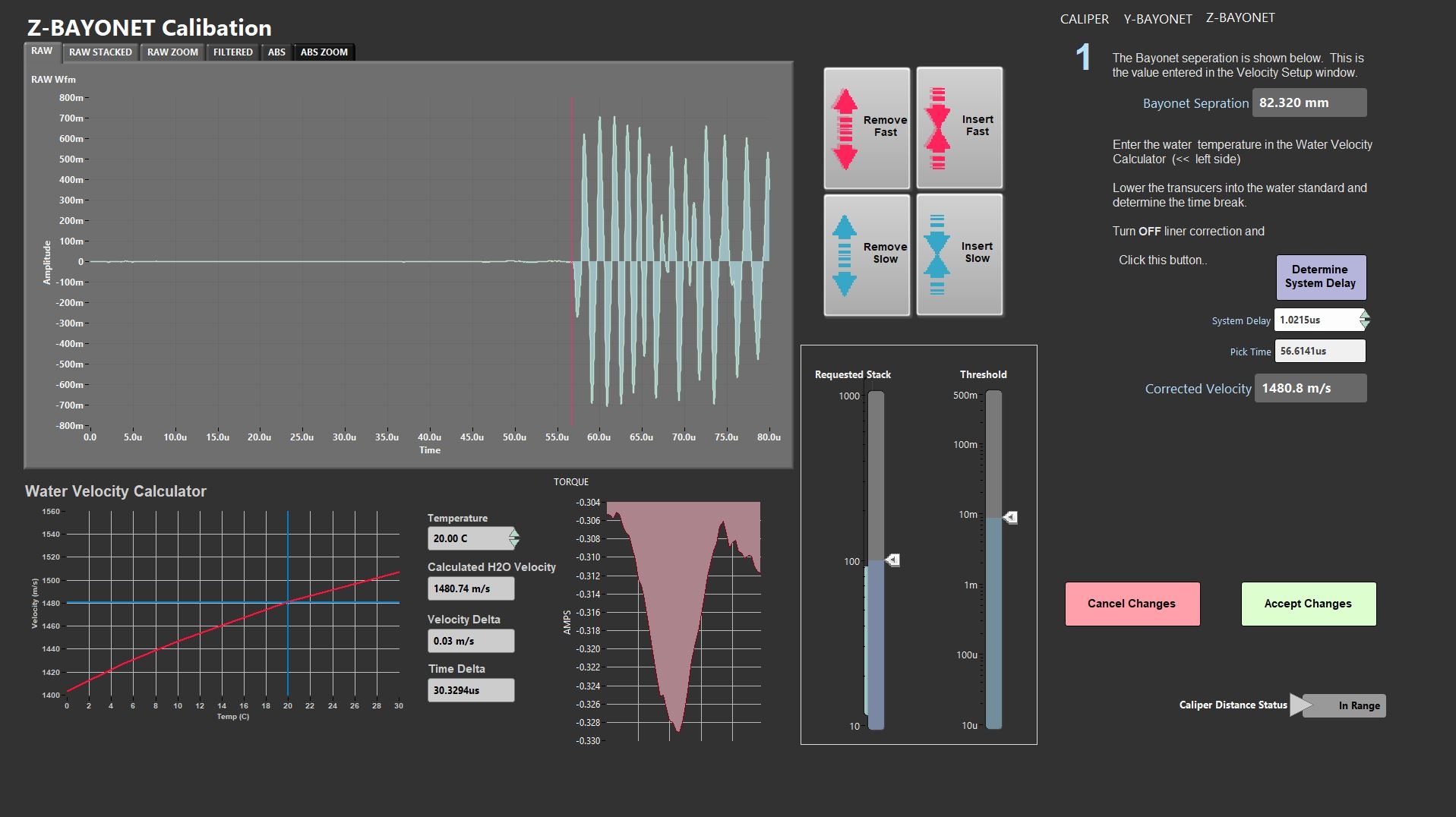
Figure 12. Y-bayonet and Z-bayonet Calibration windows. Y-bayonet raw graph tab (left), Z-bayonet raw graph tab (center), Y-bayonet ABS Zoom graph tab (right).
To calibrate the bayonets:
- Fill the bayonet calibration liner with DI water (Figure 13). The water level must be high enough that the black transducer pads on the bayonets can be placed below the water line without touching the liner itself. The water should be at room temperature if possible.
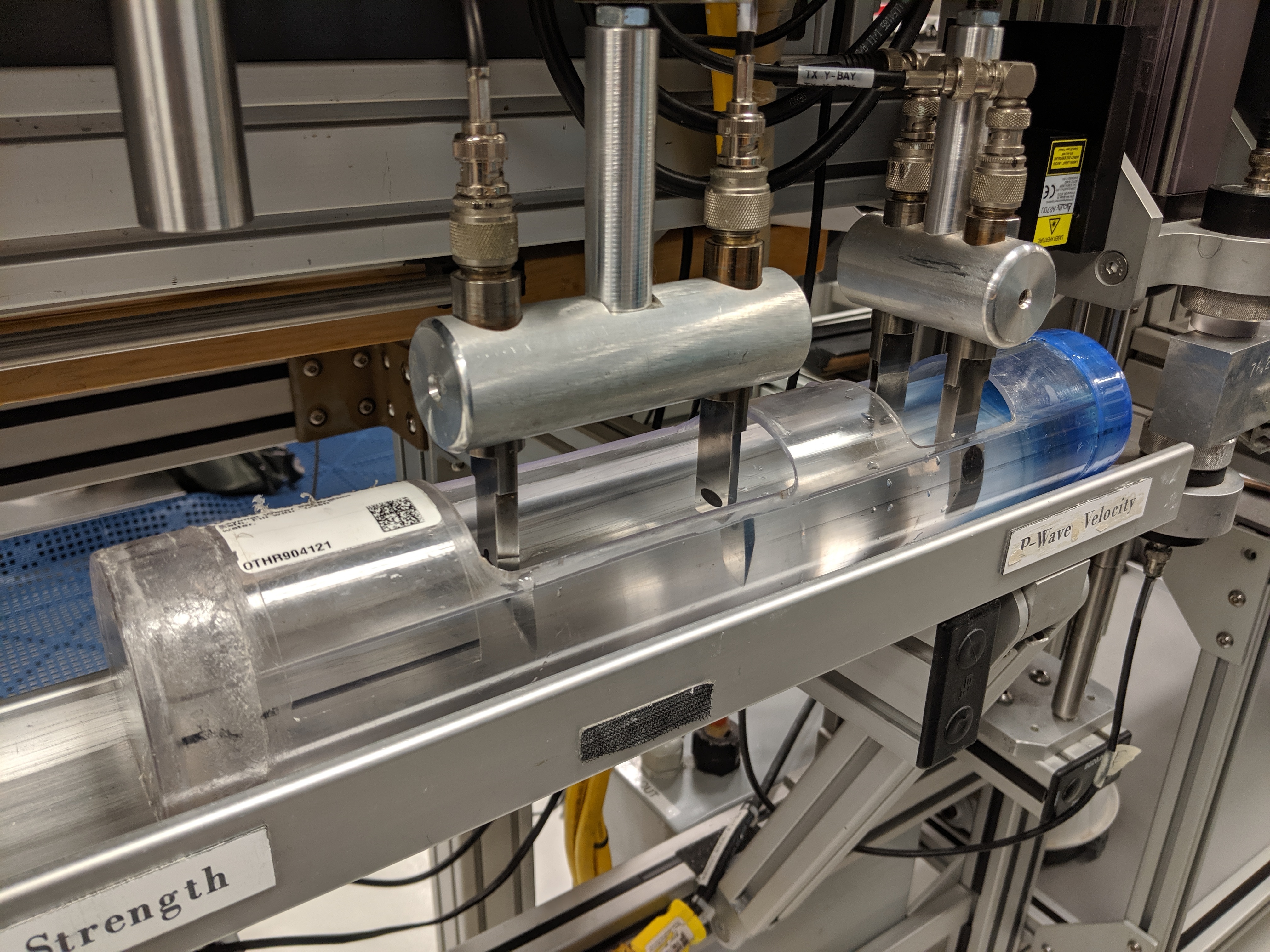
Figure 12. Bayonet Water Standard
2. Place the liner below the bayonets.
3. Open the bayonet calibration window for the selected axis
4. Verify the bayonet separation value. If the value is incorrect, go to the Velocity Setup window (Figure 13) to edit the value.
5. Use a thermometer to measure the temperature of the water in the calibration liner.
6. Enter the temperature value in the Temperature field next to the Water Velocity Calculator (lower left of the window). The screen displays a plot of theoretical velocity of water vs. temperature.
7. Use the Insert slow or Insert fast buttons to lower the bayonets into the water until the black transducer pads are submersed. Use care when lowering the Y-bayonet to ensure you do not contact the core liner.
8. Verify the software is picking the first arrival wave in the Raw Stacked graph tab. You can adjust the threshold scale bar to achieve the proper pick location (Figure 12) as long as the signal is not too noisy. Also, verify the auto-pick location in the Absolute Value tab (ABS or ABS Zoom) (Figure 12). This pick should be at the zero crossing after the first wave form above noise (Figure 12). An algorithm calculates the temperature-corrected velocity of the water bath and displays the result in theCorrected Velocity field.
9. Select Determine System Delay. The computer calculates the system delay based on the separation distance and theoretical velocity of water.
10. Compare the corrected velocity to the calculated H20 velocity value. If the values are not within range, redo the calibration.
11. Select Accept Changes to save the calibration or select Cancel Changes to leave without saving the calibration.
12. As a check on your calibration, measure the velocity of the water to verify it is within an expected error margin, +/- 2.0%. Ensure the proper sample type is selected when verifying the calibration.
C. Set Measurement Parameters
Configuration values should be set during initial setup and configuration by the physical properties technician. There should be no need to change these values unless the configuration files is corrupted. This window allows the user to view and modify the physical configuration values for the Velocity system, as well as the liner correction values and the velocity filter settings.
To open the Velocity instrument setup window (Figure 13), select Stations > Velocity Setup from the IMS panel menu (Figure 5).
- Ensure the values in the window are set as shown in Figure 13.
- Caliper and Bayonet Offsets: Physical offset from the laser zero point to the center of the transducer pair for the three stations (caliper, bayonet Y, bayonet Z). This measurement will not change unless the station location is physically changed.
- Axis Separation: Physical distance between the bayonet transducer pairs. This measurement should never change unless the bayonets holders are physically changed. The X-Axis is not shown because its separation is determined during calibration and measurement by the AR700 laser.
- Liner Correction: The liner delay value as determined experimentally based on the liner thickness and velocity measurements on the liner material.
- Velocity Disable "Save" Filter: When the filter is enabled, the save feature is inactive for any automatic velocity picks outside of the velocity range set.
- Click Ok to accept to save the changes and write them to the configuration file. Click Cancel to revert to previous values. NOTE: Only one configuration file exists in the IMS folder. Every save will overwrite the config file.
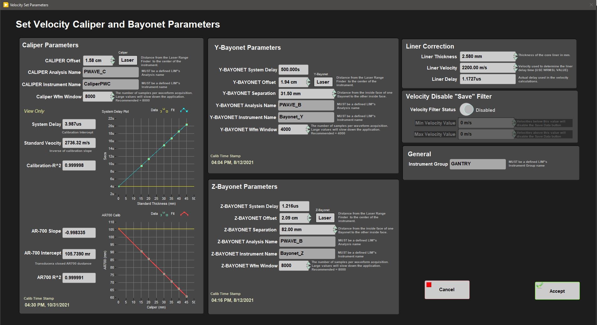
Figure 13. Velocity Parameters Window
D. Preparing Sections & Samples
A temperature-equilibrated split core section-half in it's liner is placed on the core track. The user positions the section half under the sensor, places a small piece of glad wrap on top of the core, and triggers the measurement from the software control panel. The measurement is taken continuously, with the recorded result representing the average of several thousand determinations.
On semi-lithified and lithified samples, loose material may be present on the core cut surface. Before placing the working half in the core tray, make sure the surface is clean (lightly brush away any material with a Kimwipe or paper towel).
A barcode reader records all relevant sample information, which is used for the data upload into LIMS. A laser sensor measures the distance to the top of the section-half and determines the sampling interval from the known sensor offsets.
Discrete measurements are discussed in the Caliper Measurement section below. When inserting the bayonets or closing the calipers into/on a sample, the graph should be monitored for signal quality.
Caliper Measurement
- The sample is placed between 2 flat, 1 inch diameter sensors that squeeze firmly onto the specimen to ensure good contact. De-Ionized (DI) Water is introduced between the sample and sensors to aid in signal propagation. For section-half measurements, place a small piece of Glad Wrap over the desired Caliper measurement location. This will keep the transducers clean.
- One sensor acts as a transducer and the other as a receiver to record velocity measurements at a rate of 0.5 MHz.
- To measure discrete samples in multiple axis, the sample is rotated by the user to each axis (x, y, and z-axis) and measured separately.
Bayonet Measurement
- Two pairs of piezoelectric transducers, set at 90° to each other, are inserted into the unconsolidated or semi soft section-half sediment. The sensors (black circles) must be at least partially buried in the material.
- One of each pair of sensors acts as transducer and the other as receiver to measure velocity in two directions simultaneously.
Data Quality
Velocity data quality is affected by several variables. The signal quality and pick locations should be consistently monitored by the user during every measurement.
- Quality of the acoustic coupling between the core material and the sensor transducers. Note: Use water to increase the quality of the contact.
- Quality of the coupling between both the transducer and the core liner and between the core liner and sample. Note: Use water to increase the quality of the contact.
- Consolidation of the sediments; non-cohesive sediments containing microcracks or gas voids cannot be measured accurately.
E. Making a Measurement
When scanning label barcodes on the gantry system, there are specific label types that work best.
For measurements with the bayonets and the caliper on a section half, user must use a section half label.
For measurements on discrete samples we recommend label types: Mad Residue Small, PMAG Cube label (sample type must be CUBE, CYL, or OTHR), Mad Residue Large, or Sample Table labels (the large format). Other label formats may not parse properly. Note that the MAD label parsing expects the container number in the name field. If the name field is populated with other text, the label parsing may fail.
For discrete samples shared between MAD and PMAG, use the PMAG Cube label or a sample table label. Mad residue labels WILL NOT parse for shared samples.
Currently the instrument is being upgraded, some of the measurement options or sample information input are not available.
a) Caliper Measurements
The caliper can be used to measure section half and discrete cube samples. Before measuring samples, be sure the samples are properly prepared and the system is calibrated. Retaining the correct "up" direction is critical for axis determination, and for other systems like P-mag orientation; make sure the sample has the "up" direction marked on it.
Section halves measured on the Caliper station are working half sections placed on the track with the blue end cap (top of section) toward the AR1000 laser. The laser measures the distance to the top of the section and the software calculates the offset to the measurement based on the known section length.
Discrete samples measured on the Caliper station are hard material that has been cut from the core as cubes, minicores, or slabs. Because the material can be measured in various orientations, the user must select the measurement axis.
Traveltime is calculated as total traveltime minus x-system delay time. Discrete sample measurements are not corrected for the core liner. The offset recorded in LIMS is the top offset of the discrete sample. The AR1000 laser is not used for discrete measurements. The transducer separation is measured with the displacement laser, as it is for the sample half measurement. For discrete samples the axis of measurement is selected for each measurement.
Section Half Measurement Procedure
- Place section half below the caliper. Take care to not drag the core against the bayonets while placing the core on the track.
- Place a drop of distilled water below the section on the transducer and on top of a piece of Glad Wrap on top of the section to improve contact between the caliper and section. Note: Placing Glad Wrap is not required. This is only to improve signal quality.
- Select the proper instrument and measurement axis button (Caliper SHLF X-axis)
- Close the transducer onto the core until contact is made. Do not over close the caliper on the section half.
- Verify the automatic velocity pick in the Raw Stacked graph tab (Figure 4). You can adjust the threshold scale bar to achieve the proper pick location as long as the signal is not too noisy. The user may want to verify the auto-pick location in the Absolute Value tab (ABS or ABS Zoom). This pick should be at the zero crossing after the first wave form.
- Select Save Data. A sample information window will appear (Figure 14).
- Scan the section half barcode label to populate the fields of the sample information box.
- Verify the measurement offset.
- If the offset is incorrect, select CANCEL, or enter the offset manually. The laser range finder sometimes struggles to return a proper offset if the end cap is not opaque or if the core is not flat on track. Try adding a post it note or opaque end cap to the section half if the laser returns the wrong offset.
- Select SAVE DATA.
This procedure can also be used for whole rounds or pieces of section halves, but this is rarely used. The software assumes that the whole round piece or section half piece is not within a core liner and will not correct for a liner velocity. Scan the section half label when entering the sample ID information.
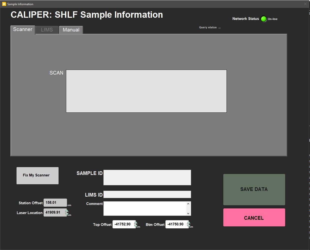
Figure 14. Section Half Caliper Measurements Sample Information Window
Discrete Sample Measurement Procedure
For each axis to be measured:
- Place a small drop of water on the lower caliper transducer
- Place the discrete sample on the caliper and add a drop of water to the top of the sample
- Select the proper instrument and measurement axis button (Caliper X-Axis, Caliper Y-Axis, Caliper Z-Axis).
- Lower the upper caliper transducer onto the specimen. Do not apply unnecessary force on the specimen as it may fracture, or cause physical variation in the caliper system and measurement.
- Verify the automatic velocity pick in the Raw Stacked graph tab (Figure 4). You can adjust the threshold scale bar to achieve the proper pick location, or pause the system to do a manual pick. The user may want to verify the auto-pick location in the Absolute Value tab (ABS or ABS Zoom). This pick should be at the zero crossing after the first wave form.
- Select Save Data. The sample information window will open (Figure 15). Note that the measurement offset will not be populated. The laser range finder is not used for discrete measurements.
- Scan the discrete sample barcode label to populate the fields of the sample information box. The sample's top offset in the section-half will be used as the measurement location, enter it manually.
- Select Save Data.
If the material to be measured is a whole piece removed from the liner (rarely used), select Caliper Piece X-Axis in Step 3. The measurement offset field in the sample information window is selectable. Scan a section half label and enter the offset of your measurement from top of the core.
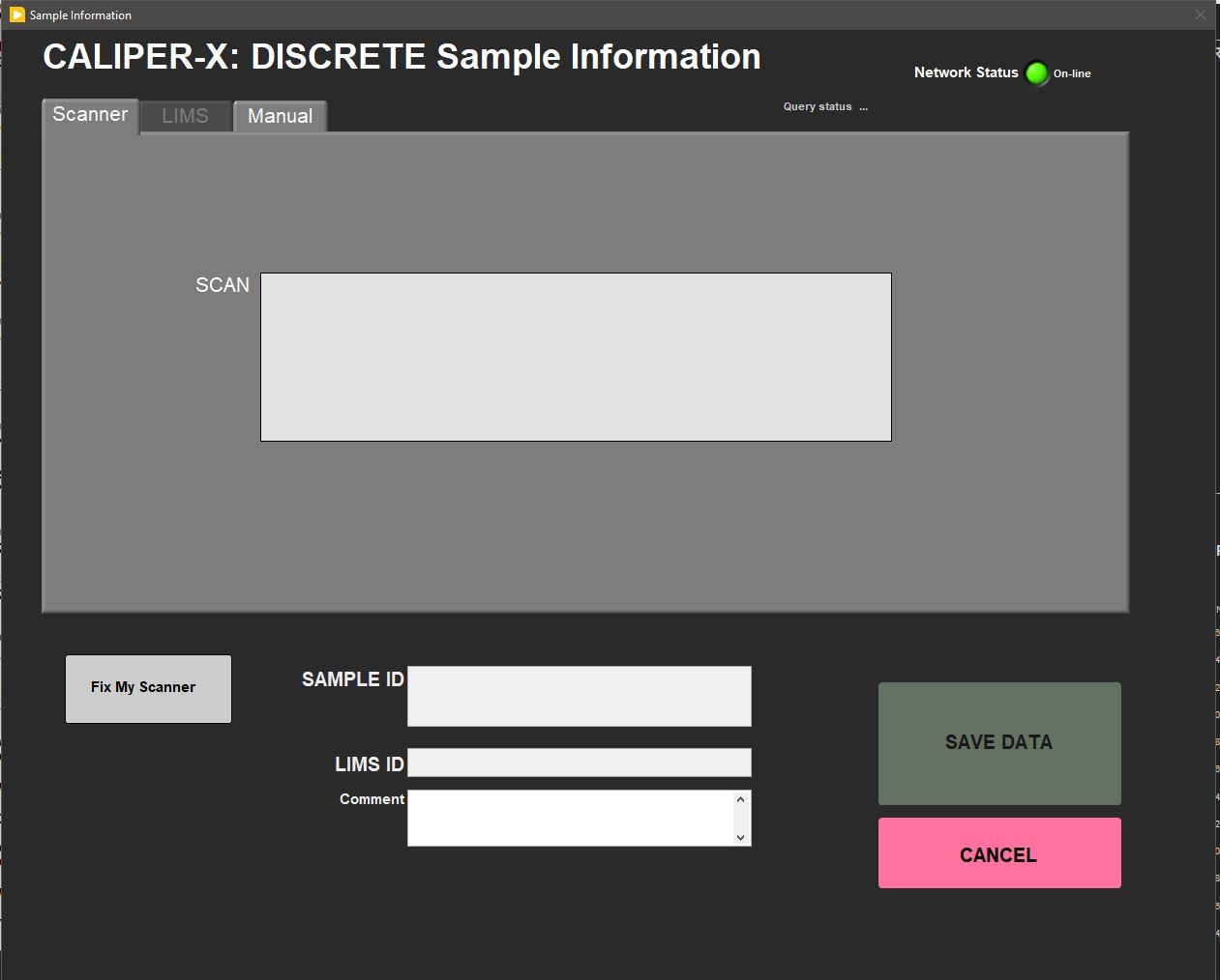
Figure 15. Discrete Caliper Measurements Sample Information Window
b) Bayonet Measurements
Before measuring samples, be sure the samples are properly prepared and the system is calibrated.
- Place section half below the bayonets. Take care to not drag the core against the bayonets while placing the core on the track.
- Select the proper instrument and measurement axis button (Y or Z bayonet)
- Lower the selected bayonets into the section half until the black transducers are below the sediment surface. A piece of glad wrap can be placed on the cut surface before inserting the bayonets, with water then added to aid in signal propagation. The glad wrap is to prevent water from being absorbed into the material.
- Verify the automatic velocity pick in the Raw Stacked graph tab (Figure 12). You can adjust the threshold scale bar to achieve the proper pick location, or pause the system to do a manual pick. The user may want to verify the auto-pick location in the Absolute Value tab (ABS or ABS Zoom). This pick should be at the zero crossing after the first wave form above noise.
- Select Save Data. A sample information window will appear (Figure 14).
- Scan the section half barcode label to populate the fields of the sample information box.
- Verify the measurement offset.
- If the offset is incorrect, select Cancel and select Save Data again, or insert it manually. The laser range finder sometimes struggles to return a proper offset if the end cap is not opaque or if the core is not flat on track. Try adding a post it note or opaque end cap to the section half if the laser returns the wrong offset.
- Once the measurement offset is verified.
- Select Save Data.
c) Manual Pick
In some cases, a user may wish to make a manual pick. This usually occurs because the automatic pick is unsuccessful, often due to a noisy signal.
Often, the Save Data option will not be available for a bad automatic velocity pick, because the values are outside of the velocity filter range. Figure 16 shows an example of a situation in which adjusting the threshold value could not overcome a large peak at the start of the measurement. Using the manual pick, the user is able to override the computers pick. Both the automatic velocity pick and manual pick are recorded in LIMS. This option is available for all measurements on the Velocity-Gantry track.
IMPORTANT: It is important that all users, on both shifts, agree ahead of time on the proper manual pick location. If they do not, each user is likely to induce a small offset in velocity due to inconsistent pick locations; the zoom tools in the lower left of the graph may help better locate the wave forms. First arrival location (Figure 17) is not as straight forward as one might assume.
The manual pick location should be relatively obvious so anyone can see it above the noise, because noise is likely to be high when auto-pick doesn't work. Then any necessary offset to correct can be applied in post processing. The agreed upon manual pick location and any offset correction in first arrival should be documented in the scientists' methods section.
To make a manual pick:
- Place sample in the selected instrument
- Once a signal is visible on the graphical display, select the Pause button in the lower left corner of the main window (Figure 4).
- The manual pick tab will be displayed on the screen (Figure 16).
- Slide the red line along the x-axis to the desired pick location. The line should be placed at the first arrival. To help select the first arrival, the plot can be zoomed in using the graph palette zoom function in the lower left corner of the graphical display.
- Verify the Velocity-manual value is reasonable for the material measured.
- Select Save Data. The sample information window will open.
- Scan the sample barcode label and save the data to the LIMS database.
To exit the manual pick and return to the automatic velocity pick, press the Play button.
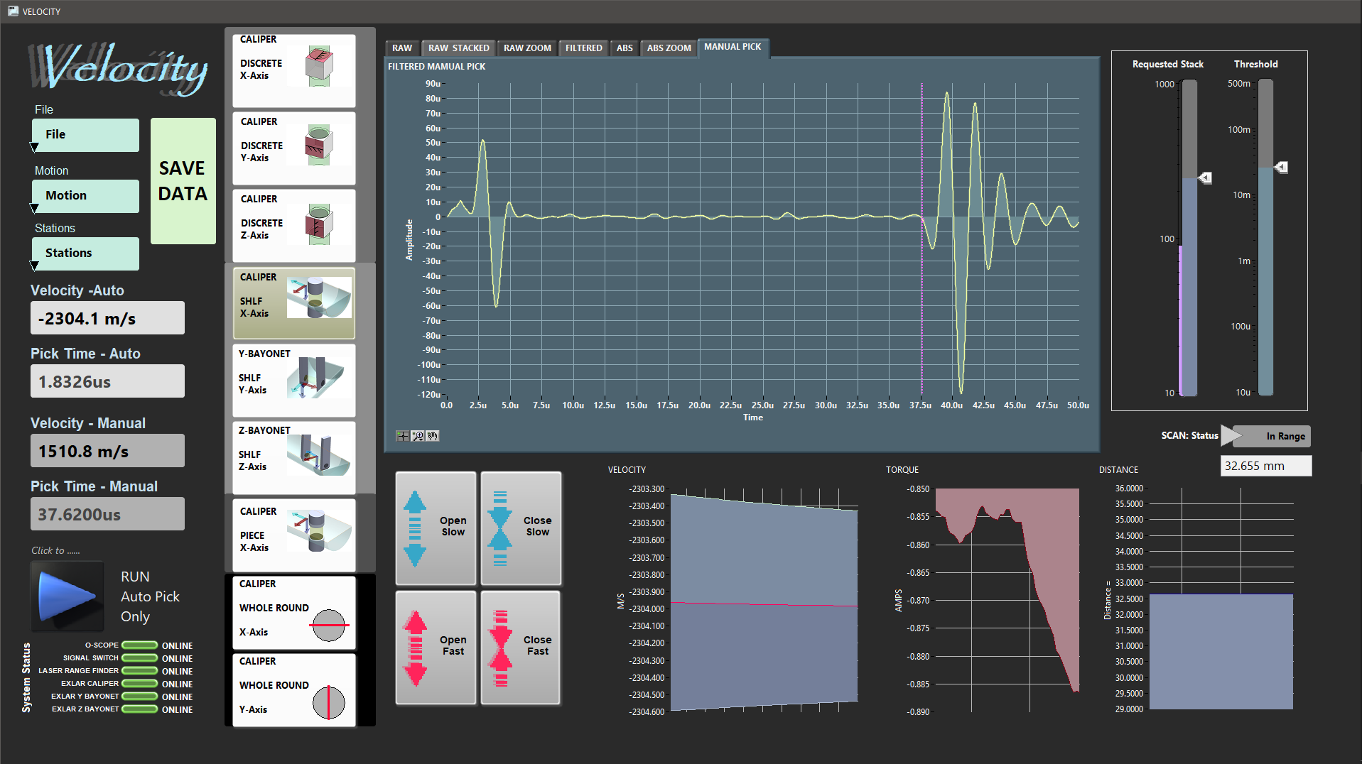
Figure 16. Manual Pick Graphical Display
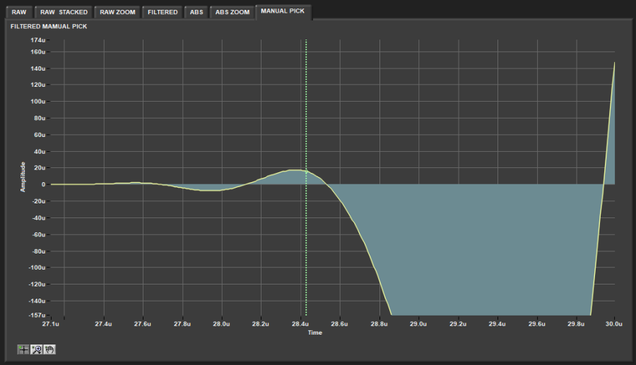
Figure 17. Zoomed Manual Pick Graphical Display
F. Evaluating your Measurement
Running a Standard as a QAQC Check
You can run a standard to verify if the instrument is measuring correctly. There are three materials available as a standard: Aluminum and acrylic are used on the caliper, and a core liner with D.I. water on the bayonets.
Expected velocities for each standard:
Aluminum 6295 m/s (+/- 63 m/s)
Acrylic 2730 m/s (+/- 27 m/s)
Water 1480 m/s (+/- 7 m/s)
Typical allowable deviation is 1% for the caliper and 0.5% for the bayonets. There will also be differences based on temperature, especially for water and aluminum. If the standard values are out of this range, ask a technician to help calibrate the instrument.
G. IMS Utilities
a) Motion Utilities
The available motion utilities are found under the Motion menu from the IMS panel menu (Figure 5).
The user may home each instrument separately using the Home Caliper, Home Y-Bayonet, Home Z-Bayonet options or home both bayonets and the caliper at the same time using the Home All command.
b) AR1000 Laser Utility
To open the AR1000 utility window (Figure 18), select Motion> AR1000 Utility from the IMS panel menu (Figure 5). This utility is useful when a user is trying to determine if the laser is correctly reading the distance to the center of each instrument.
If the mean distance shown does not agree with the instrument offset in the Velocity Setup Window (Figure 13), the offsets reported in the database will be incorrect.
The utility immediately begins reading the AR1000 laser output and averaging the values collected once the utility is opened.
To check the instrument offsets, place an object in the center of the instrument in question, i.e. the caliper. The object surface should be at the center of the instrument. An end cap works well as long as it is opaque. A tape measure can also be used to independently verify the offset value.
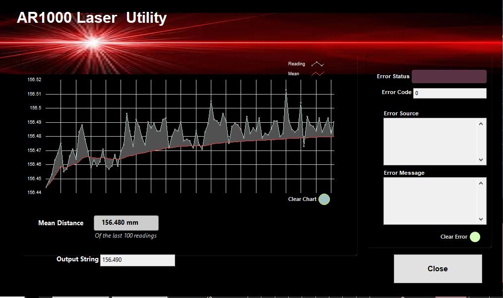
Figure 18. AR1000 Laser Utilty.
c) AR700 Displacement Laser Utility
To open the AR700 utility window (Figure 19), select Stations> AR700 Utility from the IMS panel menu (Figure 5).
Use this utility to determine if the AR700 displacement laser is returning accurate distances. The readings from this laser are used as the distance values in the velocity calculations. Inaccurate readings from the laser will cause error in the velocity readings.
The AR700 is mounted on the Caliper actuator. The more the Caliper is closed, the smaller the laser distance returned. It is recommended that the objects used for testing are similar in size to the samples being measured.
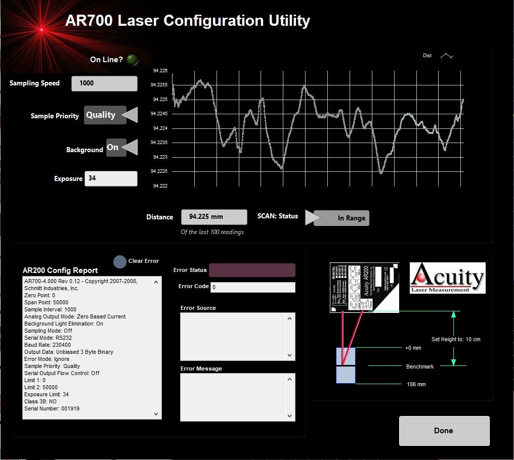
Figure 19. AR700 Displacement Laser Utility.
d) EXLAR Utility
This utility allows to control the movement and change the parameters of the three Exlar actuators: Bayonet Z, bayonet Y and Caliper.
To open it, on the main window, go to: Motion > EXLAR Utility. TRITEX Configuration Utility window will open (Figure 20).

Figure 20.- TRITEX Configuration Utility window. CONTROL tab.
The EXLAR actuator setup is saved in three different places: The actuator, the software and the Utility. The Utility is the interface between the Actuator and the software.
ACTUATOR DOWNLOAD: Copies the information from Edit Me (Utility) to the actuator.
COPY DEFAULT to EDIT ME: Copies the information from the software to the utility.
COPY ACTUATOR to EDIT ME: Copies the information from the actuator to the utility.
SYNC ALL: Copies the information from the utility to both, sofware and actuator.
CANCEL RESTORE ORIGINAL: Returns to the software setup.
DONE: Exits utility.
CALIPER: Select it if you want to work with caliper setup.
Y-BAYONET: Select it if you want to work with Y-bayonet setup.
Z-BAYONET: Select it if you want to work with z-bayonet setup.
CONTROL: Allows to move the actuator and set upper and lower limit. Could be used for testing and troubleshooting purposes.
EDIT ME: Allows to edit the utility setup information.
ACTUATOR-VIEW ONLY: Shows the information saved on the utility. To edit it the user should go to EDIT ME tab.
CONTROL tab
MOVE 1: Used for auto clamping/ insertion move.
MOVE 2: Used for removal/ unclamp.
MOVE 3: Not used by the program.
MOVE 4: Used for Emergency opening (quick unclamp/removal).
HOME: Moves the actuator to the home position.
JOG UP: Moves the actuator up (opening).
JOG DOWN: Moves the actuator down (closing).
DEF HOME: Sets the information for the home position.
RESET FAULTS: ???
DISABLE NEG LIMIT: Disable negative limit written in the box.
DISABLE POS LIMIT: Disable positive limit, written in the box.
SET NEG LIMIT: Positions the Upper actuator limit.
SET POS LIMIT: Positions the Lower actuator limit.
Negative Limit box: Selected upper limit.
Positive Limit box: Selected lower limit.
JPG SPD box: If checked, jog movements are FAST. If unchecked movements are SLOW.
MOVE TYPE box: If checked, move buttons motion is MAINTAINED. If unchecked is MOMENTARY.
STOP: Stops de movement. ???
PAUSE: Pause the movement. ???
Position: Position of the caliper or bayonet, counting from the home position.
Velocity: Speed of the movement, measured in REV/S
Current: Measured in Amp.
Caliper Compression switch State: Indicates if the caliper is under pressure.
Position, Velocity and Current graphs: Show the evolution and characteristics of the actuator movement.
ACTUATOR STATUS tab (Figure 21)
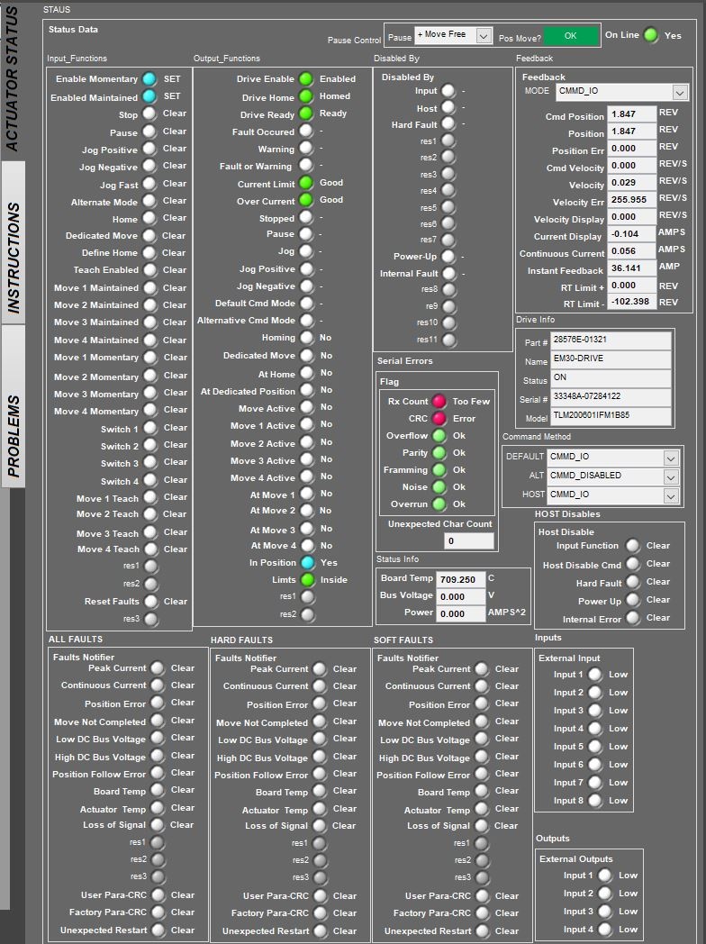
Figure 21: Actuator Status. EXLAR Utility.
Input_Functions: List of commands directed to the actuator
Output_Functions: Information related with the position and behavior of the actuator.
Disabled by: ???
Feedback: Setup information ???
Drive Info: Vendor's information about the actuator
ALL FAULTS: List of possible faults
HARD FAULTS: Hardward derived faults list.
SOFT FAULTS: Software derived faults list.
Serial Errors: ????
Status Info: Info of temperature, voltage and power.
Command Method: Command user to move the actuator.
HOST Disables: ???
Inputs: Controls set to monitor the actuator behavior. Ex: Input 1 switched ON, means that the actuator is at home position. Input 5 ON means that the caliper pressure limit switch is triggered.
Outputs: ???
ACTUATOR - VIEW ONLY tab (Figure 22)
Default parameters Setup for the caliper actuator are shown in Figure 22.

Figure 22. Caliper, actuator - view only Setup. EXLAR Utility.
The ACTUATOR - VIEW ONLY diagram shows the default setup for each one of the actuators.
All the characteristics of the different types of movements that the actuators execute are defined here.
There are different setups for each one of the actuator. See Figure 23 and 24 for Bayonets setup.
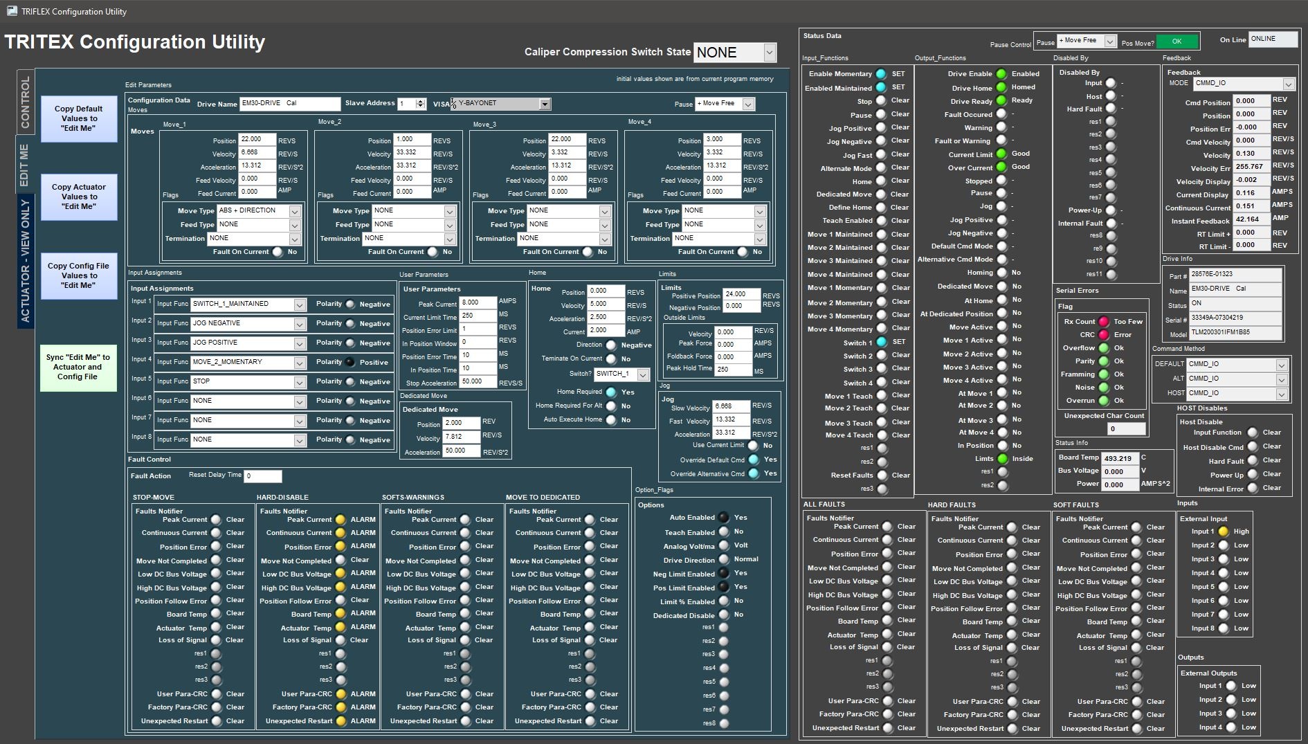
Figure 23. Y-Bayonet actuator - view only Setup. EXLAR Utility.

Figure 24. Z-Bayonet actuator - view only Setup. EXLAR Utility.
EDIT ME tab
It presents the same configuration as the ACTUATOR - VIEW ONLY tab. On this diagram the user can define or change the behavior of each one of the movements defined for the actuator.
In order to save the changes the information must be transferred to the actuator, the software or to both of them. For this purpose, use the buttons on the left side of the window.
III. Uploading Data to LIMS
A. Data Upload Procedure
To upload the images into the database (LIMS) MegaUploadaTron (MUT) program must be running in background.
If not already started do the following:
- On the desktop click the MUT icon on the bottom task bar (Figure 25) and login with ship credentials. The LIMS Uploader window will appear (Figure 26).
- Once activated, the list of files from the C:\DATA\IN directory is displayed. Files are marked ready for upload by a green check mark.

Figure 25. MUT icon
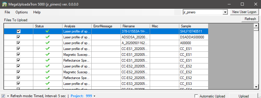
Figure 26. LIMS Uploader window
3. To manually upload files, check each file individually and clip upload. To automatically upload files, click on the Automatic Upload checkbox. The window can be minimized and MUT will be running in the background.
4. If files are marked by a purple question mark or red and white X icons, please contact a technician.
Purple question mark: Cannot identify the file.
Red and white X icons: Contains file errors.
5. Upon upload, data is moved to C:\DATA\Archive. If upload is unsuccessful, data is automatically moved to C:\DATA\Error. Please contact the PP technician is this occurs.
Data File Formats
The files generated by the Velocity Gantry system are:
- Velocity.ini: A file containing the configuration information for each instrument on the Velocity Gantry track and the most recent calibration information for each instrument
- .pwc: A file containing an individual measurement on the Caliper or Bayonets. Data includes distance between calipers (mm), travel time (us), the measurement offset on the section (cm) (no offset included for discretes), the calculated velocity (m/s), the time stamp of the measurement, the system delay, and the liner time correction. The name and location of all associated files are also listed within this file.
- .lvm: A file containing the transducer signal data for the given measurement. The signal and time (us) are provided.
B. View and Verify Data
Data Available in LIVE
The data measured on each instrument can be viewed in real time on the LIMS information viewer (LIVE).
Choose the appropriate template (Ex: PHYS_PROPS_Summary), Expedition, Site, Hole or the needed restrictions and click View Data. The requested data will be displayed. You can travel in them by clicking on each of each core or section, which will enlarge the image.
Data Available in LORE
The data for the P-wave velocity Caliper System (PWC) and P-wave velocity Bayonets System (PWB) are each displayed under a different report in LORE. These reports are found under the Physical Properties heading. The expanded reports include the linked original data files and more detailed information regarding the measurement.
P-Wave Velocity, Caliper System (PWC) Standard Report
- Exp: Expedition number
- Site: Site number
- Hole: Hole number
- Core: Core number
- Type: Type indicates the coring tool used to recover the core (typical types are F, H, R, X).
- Sect: Section number
- A/W: Archive (A) or working (W) section half.
- Offset on section (cm): Position of the sample being measured relative to the top of a section or section half.
- Offset (cm): Position of observation made on a sample (typically a section half), measured relative to the top of the sample.
- Depth CSF-A (m): Location of the observation expressed relative to the top of a hole.
- Depth [other] (m): Location of the observation expressed relative to the top of a hole. The location is presented in a scale selected by the science party or the report user.
- P-wave velocity x|y|z|unknown (m/s): Velocity of pressure wave through sample along the noted axis.
- Caliper separation (mm): Displacement between the faces of the transducers in contact with the sample, associated with the velocity observation in the specified axis.
- Sonic traveltime (µs): Traveltime of the sonic wave from transducer to transducer through the sample, associated with the velocity observation in the specified axis.
- P-wave velocity x|y|z|unknown [manual] (m/s): Velocity of pressure wave through sample in the noted axis, calculated using the manually picked traveltime.
- Sonic traveltime [manual] (µs): Manually picked traveltime of the sonic wave from transducer to transducer through the sample, associated with the velocity observation in the specified axis.
- Timestamp (UTC): Point in time at which the data was uploaded on the Gantry.
- Instrument: An abbreviation or mnemonic for the P-wave sensing device used to make these observations (CaliperPWS).
- Instrument group: Abbreviation or mnemonic for the data collection device used to acquire this observation (Gantry).
- Text ID: Automatically generated unique database identifier for a sample, visible on printed labels.
- Test No: Unique number associated with the instrument measurement steps that produced these data.
- Comments: Observer's notes about a measurement, the sample, or the measurement process.
P-Wave Velocity, Bayonet System (PWB) Standard Report
- Exp: Expedition number
- Site: Site number
- Hole: Hole number
- Core: Core number
- Type: Type indicates the coring tool used to recover the core (typical types are F, H, R, X).
- Sect: Section number
- A/W: Archive (A) or working (W) section half.
- Offset on section (cm): Position of the sample being measured relative to the top of a section or section half.
- Offset (cm): Position of observation made on a sample (typically a section half), measured relative to the top of the sample.
- Depth CSF-A (m): Location of the observation expressed relative to the top of a hole.
- Depth [other] (m): Location of the observation expressed relative to the top of a hole. The location is presented in a scale selected by the science party or the report user.
- P-wave velocity x|y|z|unknown (m/s): Velocity of pressure wave through sample along the noted axis.
- Caliper separation (mm): Displacement between the faces of the transducers in contact with the sample, associated with the velocity observation in the specified axis.
- Sonic traveltime (µs): Traveltime of the sonic wave from transducer to transducer through the sample, associated with the velocity observation in the specified axis.
- P-wave velocity x|y|z|unknown [manual] (m/s): Velocity of pressure wave through sample in the noted axis, calculated using the manually picked traveltime.
- Sonic traveltime [manual] (µs): Manually picked traveltime of the sonic wave from transducer to transducer through the sample, associated with the velocity observation in the specified axis.
- Timestamp (UTC): Point in time at which the data was uploaded on the Gantry.
- Instrument: An abbreviation or mnemonic for the P-wave sensing device used to make these observations (CaliperPWS).
- Instrument group: Abbreviation or mnemonic for the data collection device used to acquire this observation (Gantry).
- Text ID: Automatically generated unique database identifier for a sample, visible on printed labels.
- Test No: Unique number associated with the instrument measurement steps that produced these data.
- Comments: Observer's notes about a measurement, the sample, or the measurement process
C. Retrieve Data from LIMS
Expedition data can be downloaded from the database using the instrument Expanded Report on Download LIMS core data (LORE).
IV. Important Notes
Standards
Various standards are available for the P-Wave Gantry system (Figure 27). These include:
- Laboratory reagent water (distilled) (for the bayonet calibration), velocity = 1480 m/s at 20 degrees C
- Aluminum block of known length and velocity; velocity = 6295 m/s (for caliper calibration)
- Acrylic half-cylinders of variable thicknesses; the assumed Acrylic Velocity as of June, 2019 is 2730 m/s.
- Liner Velocity accepted value as of June 2019 is 2100 m/s with 40 m/s error
It is recommended that the check standard used be similar in size to the sample being measured.
Figure 27. Velocity Standards.
V. Appendix
A.1 Health, Safety & Environment
Safety
- Keep extraneous items and body parts away from the moving parts.
- The track system has three emergency opening buttons, one on the top of each actuator (Figure 28). Pressing the emergency opening button will open the actuator.
- Do not look directly into the laser light source (class 2 laser product).
- Do not direct the laser beam at other people.
- Do not attempt to work on the system while a measurement is in progress.
- Do not lean over or on the track.
- Do not stack anything on the track.
- This analytical system does not require personal protective equipment.
Figure 28. Emergency opening buttons on the Velocity Track
Pollution Prevention
This procedure does not generate heat or gases and requires no containment equipment.
Waste Management
Dispose all the plastic wrap in an approved waste container.
A.2 Maintenance and Troubleshooting
Common Issues
The following are common problems encountered when using the P-wave Velocity Gantry and their possible causes and solutions. For information about the laser Measurement and Operation software, read Gantry NI Max setup.docx. Vp GIESA Gantry Laser Operation manual.(updating)
Issue | Possible Causes | Solution |
Laser sensor: no laser light/no laser range data | Sampling is turned off | Turn sampling on through laser Measurement and Operation software |
Power supply voltage too low | Check power supply input voltage through laser Measurement and Operation software | |
Laser sensor: Serial port not responding | Power supply voltage too low | Check power supply input voltage through laser Measurement and Operation software |
Baud rate incorrect or unknown | See Acuity manual 3.5.1; laser Measurement and Operation software | |
Laser sensor: Error code (Exx) transmitted on serial port | See Acuity manual 5.3; laser Measurement and Operation software | |
Exlar actuator: No response | I/O error | Check drive or Exlar software for faults Use MOTION1/MOTION2/JOG commands. Use arrow up to upload parameters |
Power interruption | Check wiring | |
Exlar actuator: Behaving erratically | Drive improperly tuned | Check gain settings Use MOTION1/MOTION2/JOG commands. Use arrow up to upload parameters |
Too much load on motor | Check for load irregularity or excess load | |
Exlar actuator: Cannot move load | Too much load or friction | Check load and friction sources |
Excessive side load | Check side load | |
Misalignment of output rod to load | Check alignment of rod and load | |
Current limit on drive too low | Check current on drive | |
Power supply current too low | Check power supply current | |
Exlar actuator: Housing vibrates when shaft in motion | Loose mounting | Tighten mounting screws |
Drive improperly tuned | Check gain settings | |
Exlar actuator: Output rod rotates during motion | Rod rotation prevents proper linear motion | Install anti-rotation assembly |
Exlar actuator: Overheating | Ambient temperature too high | Check ambient temperature |
Actuator operation outside continuous ratings | Check operation settings | |
Amplifier poorly tuned | Check gain settings | |
| Caliper Freezes in place | Put too much force on object and passed the current limit | Open Exlar utility and press sync to coordinate the software settings and the actuator. |
| Auto Open/Auto Close Buttons cause caliper to freeze | The rev/sec may be incorrect for the caliper | Check Exlar utilities window. Change 22 rev/sec on Motion 1 and 3 to 21 rev/sec |
Resetting the AR700 Laser Baud Rate
A common issue with the Caliper system is the AR700 laser baud rate. If power is lost to the Laser it may default to an incorrect baud rate when turned back on. See the Gantry NI Max setup.docx or find the AR700 Vendor Manual in the Lab Notebook: Physical Properties page under Resources: General section.
Maintenance
After Every Sample
Clean contact sensors with tissue, cloth, or paper towel and water.
Start of Expedition/As Needed
Remove the caliper transducer caps (clear acrylic) from the caliper by unscrewing the aluminum retaining ring. With a Kimwipe, remove all old Couplant fluid and water. Thinly coat the transducer's surface, or the cap for the upper transducer, with Couplant B, and re-screw the retaining ring. Re-calibrate after each time, paying attention to the signal quality.
Clean dust from the laser sensor lens using compressed air or delicate tissue wipes. Do not use organic cleaning solvents on the sensor lens.
Check that lower transducer for caliper is making contact with core liner as sections are measured.
Polish the transducer cap when marks are noticed. Transparent ones are polish on Thin Sections lab. Metal ones?
Annually
Coat (not pack) the following parts of the actuators with grease:
- Angular contact thrust bearings
- Roller screw cylinder
- Roller screw assembly in the actuators
Examine the cable management system for abraded cables or other indications of wear.
B.1 IMS Program Structure
a) IMS Program Structure
IMS is a modular program. Individual modules are as follows:
- Config Files: Unique for each track. Used for initialize the track and set up default parameters.
- Documents: Important Information related with configuration setup.
- Error: IMS error file.
- FRIENDS: Systems that use IMS but don't use DAQ Engine.
- IMS Common: Programs that are used by different instruments.
- PLUG-INS: Code for each of the instruments.
- Projects: Main IMS libraries.
- Resources: Other information and programs needed to run IMS.
- UI: User Interface
- X-CONFIG: .ini files, specifics for each instrument.
- MOTION plug-in: Codes for the motion control system.
- DAQ Engine: Code that organizes INST and MOTION plug-ins into a track system.
The IMS Main User Interface (IMS-UI) calls these modules, instructs them to initialize, and provides a user interface to their functionality.
The Velocity system, specifically, is built with three INST modules (Caliper, Y-Bayonet, Z-bayonet), three MOTION modules (one for each instrument actuator) .
The IMS Main User Interface (IMS-UI) calls these modules, instructs them to initialize, and provides a user interface to their functionality.
Each module manages a configuration file that opens the IMS program at the same state it was when previously closed and provides utilities for the user to edit or modify the configuration data and calibration routines.
The three buttons on the left side of the IMS-UI window provide access to utilities/editors via dropdown menus as shown in Figure 5.
b) Communication and Control Setup
Data communication and control is USB based and managed via National Instrument’s Measurement & Automation Explorer (NI-MAX). When you open NI-MAX and expand the Device and Interface section. The correct communications setup can be found at IMS Hardware Communications Setup.
B.2 Motion Control Setup
Refer to EXLAR Utility for further information.
B.3 LIMS Component Tables
The tables below contain the LIMS components for the following ANALYSIS codes:
- PWAVE_B - p-wave velocity by X- and Z-axis bayonet
- PWAVE_C - p-wave velocity by caliper (X, Y, or Z axis)
| ANALYSIS | TABLE | NAME | ABOUT TEXT |
| PWAVE_B | SAMPLE | Exp | Exp: expedition number |
| PWAVE_B | SAMPLE | Site | Site: site number |
| PWAVE_B | SAMPLE | Hole | Hole: hole number |
| PWAVE_B | SAMPLE | Core | Core: core number |
| PWAVE_B | SAMPLE | Type | Type: type indicates the coring tool used to recover the core (typical types are F, H, R, X). |
| PWAVE_B | SAMPLE | Sect | Sect: section number |
| PWAVE_B | SAMPLE | A/W | A/W: archive (A) or working (W) section half. |
| PWAVE_B | SAMPLE | text_id | Text_ID: automatically generated database identifier for a sample, also carried on the printed labels. This identifier is guaranteed to be unique across all samples. |
| PWAVE_B | SAMPLE | sample_number | Sample Number: automatically generated database identifier for a sample. This is the primary key of the SAMPLE table. |
| PWAVE_B | SAMPLE | label_id | Label identifier: automatically generated, human readable name for a sample that is printed on labels. This name is not guaranteed unique across all samples. |
| PWAVE_B | SAMPLE | sample_name | Sample name: short name that may be specified for a sample. You can use an advanced filter to narrow your search by this parameter. |
| PWAVE_B | SAMPLE | x_sample_state | Sample state: Single-character identifier always set to "W" for samples; standards can vary. |
| PWAVE_B | SAMPLE | x_project | Project: similar in scope to the expedition number, the difference being that the project is the current cruise, whereas expedition could refer to material/results obtained on previous cruises |
| PWAVE_B | SAMPLE | x_capt_loc | Captured location: "captured location," this field is usually null and is unnecessary because any sample captured on the JR has a sample_number ending in 1, and GCR ending in 2 |
| PWAVE_B | SAMPLE | location | Location: location that sample was taken; this field is usually null and is unnecessary because any sample captured on the JR has a sample_number ending in 1, and GCR ending in 2 |
| PWAVE_B | SAMPLE | x_sampling_tool | Sampling tool: sampling tool used to take the sample (e.g., syringe, spatula) |
| PWAVE_B | SAMPLE | changed_by | Changed by: username of account used to make a change to a sample record |
| PWAVE_B | SAMPLE | changed_on | Changed on: date/time stamp for change made to a sample record |
| PWAVE_B | SAMPLE | sample_type | Sample type: type of sample from a predefined list (e.g., HOLE, CORE, LIQ) |
| PWAVE_B | SAMPLE | x_offset | Offset (m): top offset of sample from top of parent sample, expressed in meters. |
| PWAVE_B | SAMPLE | x_offset_cm | Offset (cm): top offset of sample from top of parent sample, expressed in centimeters. This is a calculated field (offset, converted to cm) |
| PWAVE_B | SAMPLE | x_bottom_offset_cm | Bottom offset (cm): bottom offset of sample from top of parent sample, expressed in centimeters. This is a calculated field (offset + length, converted to cm) |
| PWAVE_B | SAMPLE | x_diameter | Diameter (cm): diameter of sample, usually applied only to CORE, SECT, SHLF, and WRND samples; however this field is null on both Exp. 390 and 393, so it is no longer populated by Sample Master |
| PWAVE_B | SAMPLE | x_orig_len | Original length (m): field for the original length of a sample; not always (or reliably) populated |
| PWAVE_B | SAMPLE | x_length | Length (m): field for the length of a sample [as entered upon creation] |
| PWAVE_B | SAMPLE | x_length_cm | Length (cm): field for the length of a sample. This is a calculated field (length, converted to cm). |
| PWAVE_B | SAMPLE | status | Status: single-character code for the current status of a sample (e.g., active, canceled) |
| PWAVE_B | SAMPLE | old_status | Old status: single-character code for the previous status of a sample; used by the LIME program to restore a canceled sample |
| PWAVE_B | SAMPLE | original_sample | Original sample: field tying a sample below the CORE level to its parent HOLE sample |
| PWAVE_B | SAMPLE | parent_sample | Parent sample: the sample from which this sample was taken (e.g., for PWDR samples, this might be a SHLF or possibly another PWDR) |
| PWAVE_B | SAMPLE | standard | Standard: T/F field to differentiate between samples (standard=F) and QAQC standards (standard=T) |
| PWAVE_B | SAMPLE | login_by | Login by: username of account used to create the sample (can be the LIMS itself [e.g., SHLFs created when a SECT is created]) |
| PWAVE_B | SAMPLE | login_date | Login date: creation date of the sample |
| PWAVE_B | SAMPLE | legacy | Legacy flag: T/F indicator for when a sample is from a previous expedition and is locked/uneditable on this expedition |
| PWAVE_B | TEST | test changed_on | TEST changed on: date/time stamp for a change to a test record. |
| PWAVE_B | TEST | test status | TEST status: single-character code for the current status of a test (e.g., active, in process, canceled) |
| PWAVE_B | TEST | test old_status | TEST old status: single-character code for the previous status of a test; used by the LIME program to restore a canceled test |
| PWAVE_B | TEST | test test_number | TEST test number: automatically generated database identifier for a test record. This is the primary key of the TEST table. |
| PWAVE_B | TEST | test date_received | TEST date received: date/time stamp for the creation of the test record. |
| PWAVE_B | TEST | test instrument | TEST instrument [instrument group]: field that describes the instrument group (most often this applies to loggers with multiple sensors); often obscure (e.g., user_input) |
| PWAVE_B | TEST | test analysis | TEST analysis: analysis code associated with this test (foreign key to the ANALYSIS table) |
| PWAVE_B | TEST | test x_project | TEST project: similar in scope to the expedition number, the difference being that the project is the current cruise, whereas expedition could refer to material/results obtained on previous cruises |
| PWAVE_B | TEST | test sample_number | TEST sample number: the sample_number of the sample to which this test record is attached; a foreign key to the SAMPLE table |
| PWAVE_B | CALCULATED | Depth CSF-A (m) | Depth CSF-A (m): position of observation expressed relative to the top of the hole. |
| PWAVE_B | CALCULATED | Depth CSF-B (m) | Depth [other] (m): position of observation expressed relative to the top of the hole. The location is presented in a scale selected by the science party or the report user. |
| PWAVE_B | RESULT | config_asman_id | RESULT config file ASMAN_ID: serial number of the ASMAN link for the configuration file |
| PWAVE_B | RESULT | config_filename | RESULT config filename: file name of the configuration file |
| PWAVE_B | RESULT | distance_in_caliper (mm) | RESULT distance in caliper (mm): distance between transducers |
| PWAVE_B | RESULT | manual_pick_travel_time (µs) | RESULT manual pick travel time (us): manually picked traveltime of the sonic wave from transducer to transducer through the sample, associated with the velocity observation in the specified axis. |
| PWAVE_B | RESULT | manual_pick_velocity_y (m/s) | RESULT manual pick Y-axis velocity (m/s): velocity of pressure wave through sample for the Y axis, calculated using the manually picked traveltime. |
| PWAVE_B | RESULT | manual_pick_velocity_z (m/s) | RESULT manual pick Z-axis velocity (m/s): velocity of pressure wave through sample for the Z axis, calculated using the manually picked traveltime. |
| PWAVE_B | RESULT | observed_length (cm) | RESULT observed length (cm): length of the section as recorded by the core logger track |
| PWAVE_B | RESULT | offset (cm) | RESULT offset (cm): position of the observation made, measured relative to the top of a section half. |
| PWAVE_B | RESULT | run_asman_id | RESULT run file ASMAN_ID: serial number of the ASMAN link for the run (.PWC) file |
| PWAVE_B | RESULT | run_filename | RESULT run filename: file name of the run (.PWC) file |
| PWAVE_B | RESULT | timestamp | RESULT timestamp: date/time stamp for the actual measurement time |
| PWAVE_B | RESULT | transducer_signal_asman_id | RESULT transducer signal file ASMAN_ID: serial number of the ASMAN link for the transducer signal (.LVM) file |
| PWAVE_B | RESULT | transducer_signal_filename | RESULT run filename: file name of the transducer signal (.LVM) file |
| PWAVE_B | RESULT | travel_time (µs) | RESULT travel time (us): traveltime of the sonic wave from transducer to transducer through the sample, associated with the velocity observation in the specified axis. (Calculated by software) |
| PWAVE_B | RESULT | velocity_y (m/s) | RESULT sonic velocity Y-axis (m/s): velocity of pressure wave through sample for the Y axis, calculated by the software |
| PWAVE_B | RESULT | velocity_z (m/s) | RESULT sonic velocity Z-axis (m/s): velocity of pressure wave through sample for the Z axis, calculated by the software |
| PWAVE_B | SAMPLE | sample description | SAMPLE comment: contents of the SAMPLE.description field, usually shown on reports as "Sample comments" |
| PWAVE_B | TEST | test test_comment | TEST comment: contents of the TEST.comment field, usually shown on reports as "Test comments" |
| PWAVE_B | RESULT | result comments | RESULT comment: contents of a result parameter with name = "comment," usually shown on reports as "Result comments" |
| ANALYSIS | TABLE | NAME | ABOUT TEXT |
| PWAVE_C | SAMPLE | Exp | Exp: expedition number |
| PWAVE_C | SAMPLE | Site | Site: site number |
| PWAVE_C | SAMPLE | Hole | Hole: hole number |
| PWAVE_C | SAMPLE | Core | Core: core number |
| PWAVE_C | SAMPLE | Type | Type: type indicates the coring tool used to recover the core (typical types are F, H, R, X). |
| PWAVE_C | SAMPLE | Sect | Sect: section number |
| PWAVE_C | SAMPLE | A/W | A/W: archive (A) or working (W) section half. |
| PWAVE_C | SAMPLE | text_id | Text_ID: automatically generated database identifier for a sample, also carried on the printed labels. This identifier is guaranteed to be unique across all samples. |
| PWAVE_C | SAMPLE | sample_number | Sample Number: automatically generated database identifier for a sample. This is the primary key of the SAMPLE table. |
| PWAVE_C | SAMPLE | label_id | Label identifier: automatically generated, human readable name for a sample that is printed on labels. This name is not guaranteed unique across all samples. |
| PWAVE_C | SAMPLE | sample_name | Sample name: short name that may be specified for a sample. You can use an advanced filter to narrow your search by this parameter. |
| PWAVE_C | SAMPLE | x_sample_state | Sample state: Single-character identifier always set to "W" for samples; standards can vary. |
| PWAVE_C | SAMPLE | x_project | Project: similar in scope to the expedition number, the difference being that the project is the current cruise, whereas expedition could refer to material/results obtained on previous cruises |
| PWAVE_C | SAMPLE | x_capt_loc | Captured location: "captured location," this field is usually null and is unnecessary because any sample captured on the JR has a sample_number ending in 1, and GCR ending in 2 |
| PWAVE_C | SAMPLE | location | Location: location that sample was taken; this field is usually null and is unnecessary because any sample captured on the JR has a sample_number ending in 1, and GCR ending in 2 |
| PWAVE_C | SAMPLE | x_sampling_tool | Sampling tool: sampling tool used to take the sample (e.g., syringe, spatula) |
| PWAVE_C | SAMPLE | changed_by | Changed by: username of account used to make a change to a sample record |
| PWAVE_C | SAMPLE | changed_on | Changed on: date/time stamp for change made to a sample record |
| PWAVE_C | SAMPLE | sample_type | Sample type: type of sample from a predefined list (e.g., HOLE, CORE, LIQ) |
| PWAVE_C | SAMPLE | x_offset | Offset (m): top offset of sample from top of parent sample, expressed in meters. |
| PWAVE_C | SAMPLE | x_offset_cm | Offset (cm): top offset of sample from top of parent sample, expressed in centimeters. This is a calculated field (offset, converted to cm) |
| PWAVE_C | SAMPLE | x_bottom_offset_cm | Bottom offset (cm): bottom offset of sample from top of parent sample, expressed in centimeters. This is a calculated field (offset + length, converted to cm) |
| PWAVE_C | SAMPLE | x_diameter | Diameter (cm): diameter of sample, usually applied only to CORE, SECT, SHLF, and WRND samples; however this field is null on both Exp. 390 and 393, so it is no longer populated by Sample Master |
| PWAVE_C | SAMPLE | x_orig_len | Original length (m): field for the original length of a sample; not always (or reliably) populated |
| PWAVE_C | SAMPLE | x_length | Length (m): field for the length of a sample [as entered upon creation] |
| PWAVE_C | SAMPLE | x_length_cm | Length (cm): field for the length of a sample. This is a calculated field (length, converted to cm). |
| PWAVE_C | SAMPLE | status | Status: single-character code for the current status of a sample (e.g., active, canceled) |
| PWAVE_C | SAMPLE | old_status | Old status: single-character code for the previous status of a sample; used by the LIME program to restore a canceled sample |
| PWAVE_C | SAMPLE | original_sample | Original sample: field tying a sample below the CORE level to its parent HOLE sample |
| PWAVE_C | SAMPLE | parent_sample | Parent sample: the sample from which this sample was taken (e.g., for PWDR samples, this might be a SHLF or possibly another PWDR) |
| PWAVE_C | SAMPLE | standard | Standard: T/F field to differentiate between samples (standard=F) and QAQC standards (standard=T) |
| PWAVE_C | SAMPLE | login_by | Login by: username of account used to create the sample (can be the LIMS itself [e.g., SHLFs created when a SECT is created]) |
| PWAVE_C | SAMPLE | login_date | Login date: creation date of the sample |
| PWAVE_C | SAMPLE | legacy | Legacy flag: T/F indicator for when a sample is from a previous expedition and is locked/uneditable on this expedition |
| PWAVE_C | TEST | test changed_on | TEST changed on: date/time stamp for a change to a test record. |
| PWAVE_C | TEST | test status | TEST status: single-character code for the current status of a test (e.g., active, in process, canceled) |
| PWAVE_C | TEST | test old_status | TEST old status: single-character code for the previous status of a test; used by the LIME program to restore a canceled test |
| PWAVE_C | TEST | test test_number | TEST test number: automatically generated database identifier for a test record. This is the primary key of the TEST table. |
| PWAVE_C | TEST | test date_received | TEST date received: date/time stamp for the creation of the test record. |
| PWAVE_C | TEST | test instrument | TEST instrument [instrument group]: field that describes the instrument group (most often this applies to loggers with multiple sensors); often obscure (e.g., user_input) |
| PWAVE_C | TEST | test analysis | TEST analysis: analysis code associated with this test (foreign key to the ANALYSIS table) |
| PWAVE_C | TEST | test x_project | TEST project: similar in scope to the expedition number, the difference being that the project is the current cruise, whereas expedition could refer to material/results obtained on previous cruises |
| PWAVE_C | TEST | test sample_number | TEST sample number: the sample_number of the sample to which this test record is attached; a foreign key to the SAMPLE table |
| PWAVE_C | CALCULATED | Depth CSF-A (m) | Depth CSF-A (m): position of observation expressed relative to the top of the hole. |
| PWAVE_C | CALCULATED | Depth CSF-B (m) | Depth [other] (m): position of observation expressed relative to the top of the hole. The location is presented in a scale selected by the science party or the report user. |
| PWAVE_C | RESULT | config_asman_id | RESULT config file ASMAN_ID: serial number of the ASMAN link for the configuration file |
| PWAVE_C | RESULT | config_filename | RESULT config filename: file name of the configuration file |
| PWAVE_C | RESULT | distance_in_caliper (mm) | RESULT distance in caliper (mm): distance between transducers |
| PWAVE_C | RESULT | manual_pick_travel_time (µs) | RESULT manual pick travel time (us): manually picked traveltime of the sonic wave from transducer to transducer through the sample, associated with the velocity observation in the specified axis. |
| PWAVE_C | RESULT | manual_pick_velocity_x (m/s) | RESULT manual pick X-axis velocity (m/s): velocity of pressure wave through sample for the X axis, calculated using the manually picked traveltime. |
| PWAVE_C | RESULT | manual_pick_velocity_y (m/s) | RESULT manual pick Y-axis velocity (m/s): velocity of pressure wave through sample for the Y axis, calculated using the manually picked traveltime. |
| PWAVE_C | RESULT | manual_pick_velocity_z (m/s) | RESULT manual pick Z-axis velocity (m/s): velocity of pressure wave through sample for the Z axis, calculated using the manually picked traveltime. |
| PWAVE_C | RESULT | observed_length (cm) | RESULT observed length (cm): length of the section as recorded by the core logger track |
| PWAVE_C | RESULT | offset (cm) | RESULT offset (cm): position of the observation made, measured relative to the top of a section half. |
| PWAVE_C | RESULT | run_asman_id | RESULT run file ASMAN_ID: serial number of the ASMAN link for the run (.PWC) file |
| PWAVE_C | RESULT | run_filename | RESULT run filename: file name of the run (.PWC) file |
| PWAVE_C | RESULT | timestamp | RESULT timestamp: date/time stamp for the actual measurement time |
| PWAVE_C | RESULT | transducer_signal_filename | RESULT run filename: file name of the transducer signal (.LVM) file |
| PWAVE_C | RESULT | travel_time (µs) | RESULT travel time (us): traveltime of the sonic wave from transducer to transducer through the sample, associated with the velocity observation in the specified axis. (Calculated by software) |
| PWAVE_C | RESULT | velocity_x (m/s) | RESULT sonic velocity X-axis (m/s): velocity of pressure wave through sample for the X axis, calculated by the software |
| PWAVE_C | RESULT | velocity_y (m/s) | RESULT sonic velocity Y-axis (m/s): velocity of pressure wave through sample for the Y axis, calculated by the software |
| PWAVE_C | RESULT | velocity_z (m/s) | RESULT sonic velocity Z-axis (m/s): velocity of pressure wave through sample for the Z axis, calculated by the software |
| PWAVE_C | SAMPLE | sample description | SAMPLE comment: contents of the SAMPLE.description field, usually shown on reports as "Sample comments" |
| PWAVE_C | TEST | test test_comment | TEST comment: contents of the TEST.comment field, usually shown on reports as "Test comments" |
| PWAVE_C | RESULT | result comments | RESULT comment: contents of a result parameter with name = "comment," usually shown on reports as "Result comments" |
C.1 Hardware
Hardware
The velocity track system consists of the following components (Figure 29):
- Caliper transducers: X-axis velocity measurements
- Chisel-type transducers (bayonet transducers): Y and Z axis velocity measurements
- 3 Linear actuators: Each actuator controls the motion for one instrument
- Laser Range Finder (AR1000 laser): Used to determine offset of measurements on section halves
- Displacement Laser (AR700): Used to determine distance between caliper transducers during measurements
- Two Signal Amplifiers: One amplifier is common to all three instruments and is used to amplify the transducer signals. The second amplifier is used as a pre-amplifier for the receiving signal from the Caliper only. The Caliper returns a weaker signal than the Bayonets. By using this pre-amplifier the Caliper signal can be amplified without affecting the Bayonet measurements. If the signal is noisy or too weak, adjustments are made on only the gain dial.

Figure 29. Bayonets, caliper and displacement laser on the Gantry track (left), signal amplifier (center), and laser range finder (right).
Caliper Transducers: Panametrics-NDT Microscan Delay Line Transducers
Specification | Value |
Frequency (MHz) | 0.5 |
Element diameter (mm) | 25 |
Part number | M2008 |
Bayonet Transducers
Custom made.
Exlar Linear Actuator
Specification | Value |
Maximum radial load (lb) | 15 |
Resolution (revolution) | 0.001 |
Accuracy (revolution) | ±0.010 |
Operating temperature (°C) | 0–55 |
Model Number | TLM20-0601-1-IFM-1BS-50-AR |
Voltage (VDC) | 48 |
Current (A) | 5000 @ 10 rpm |
Acuity 1000 Laser Distance Sensor
Specification | Value |
Distance (m) | 30 |
Laser | 650 nm, 1 mW visible red |
Accuracy | ±0.12 inch (3.05 mm) |
Resolution | 0.004 inch (0.10 mm) |
Operating temperature (°C) | –10–50 |
Linearity/accuracy (mm) | ±3 |
Acuity AR700-4 Laser Displacement Sensor
Specification | Value |
|---|---|
| Model (P/N) | AR700-4 5mW (AP7020040) |
| Laser class | 3R |
Laser type | 670nm 5mW visible RED diode |
Span | 101.6 mm |
Resolution | 5.1 microns |
Operating temperature | 0 to 50°C |
Linearity/accuracy | ±31 microns |
VI. Credits
This document was written June 2019 by B. Novak and A. de Loach with contributions from G. Acton in the IODP wiki. Portions of the manual were taken from the Archived P-Wave Velocity Gantry User Guide written by T. Cobine in 2009.
All improvements to the Quick Start Guides and User Guides are a communal effort, with honorable mention to the group of LOs, ALOs, and technicians who have helped.
VII. Archived Versions
- P-Wave User Guide - 27Sept2022
- P-Wave User Guide 2020 (*.pdf)
- P-Wave Velocity Gantry: User Guide: Word file written by T. Cobine (2009-01-17), reviewed by H. Barnes and T. Gorgas, and approved by D. J. Houpt
2 Comments
Unknown User (25dbb4e563432e130164eb694216000d)
Aug 03, 2018Missing figures, will be added on X378
Unknown User (25dbb4e563432e130164eb68f519000c)
Aug 05, 2018Reviewed by Nicolette 6 August 2018