I. Introduction533px533px
The section half image logger (SHIL) takes digital images of the flat face of split cores using a line scan camera and generates RGB data. All 'Archive' section halves are imaged on the SHIL. Sediment cores are imaged as soon as possible after splitting and scraping to minimize color changes that occur through oxidation and drying. The SHIL can also be used to image the outside of a whole round hard rock section (see section 360° Imaging Hard Rock for details).
Theory of Operation
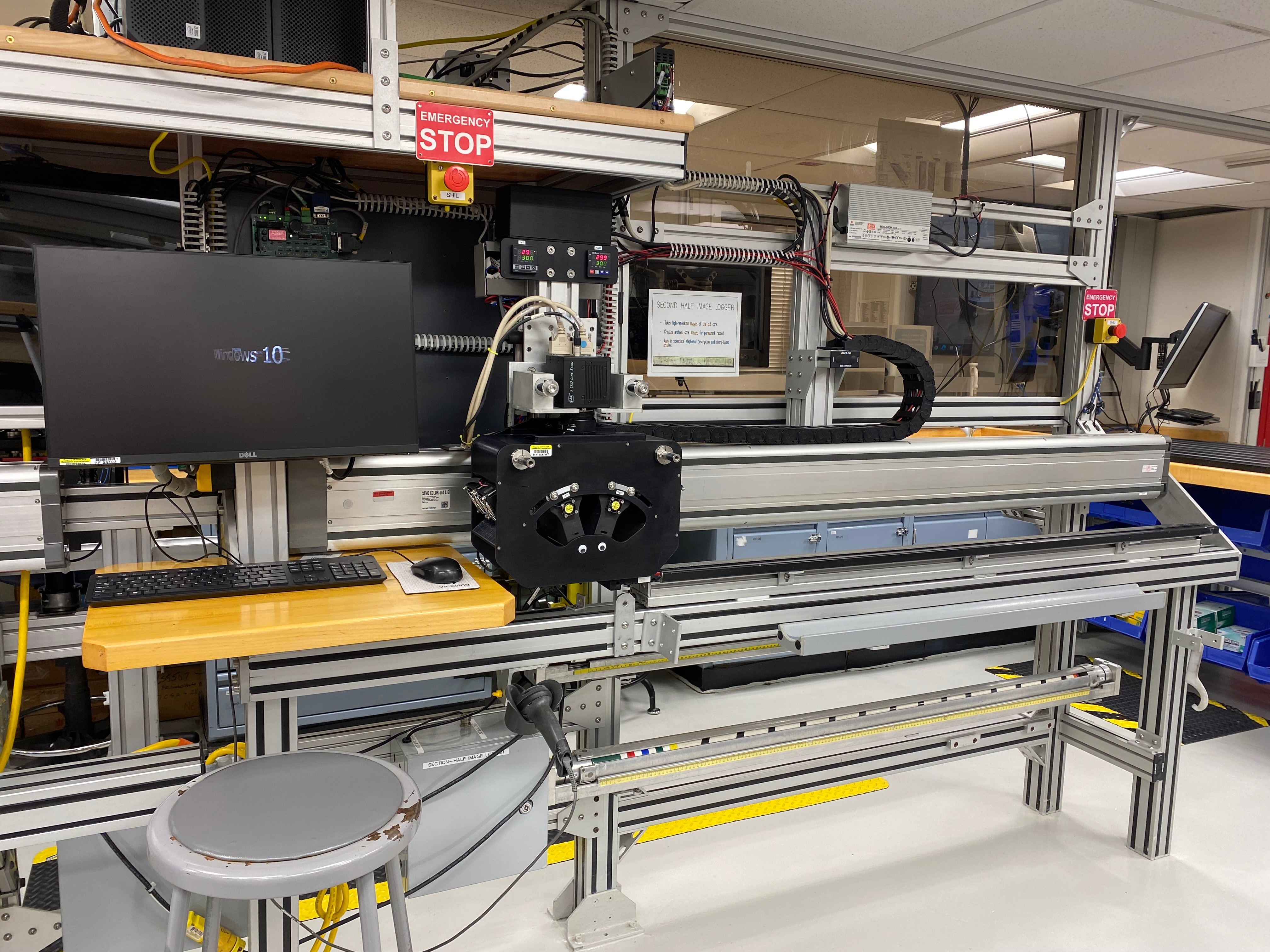
The track system is composed of two slaved linear actuators and a linear encoder that provides precise triggering pulses to a gantry-mounted JAI color line scan camera. The line scan interval is 20 lines/mm (50 microns) and the camera height is adjusted so that image pixels will be square. Light is provided by a number of Advanced Illumination high-current focused light emitting diode (LED) line lights adjusted to precise angles relative to the lens axis in order to evenly illuminate an uneven surface. Motion control is performed using Galil software and hardware coupled to the linear actuators.
Line Scan Camera
Unlike a "normal" distal photo sensor with a square sensor array, similar to a postage stamp, a line scan camera's array consists of a single line of pixels. Whereas a normal camera captures frames, the line scan camera sees only a single line at a time and sends this line image to a capture card on a dedicated computer. Line by line, the computer compiles the final image.
In some applications, the photographic subject may move in front of the camera on a conveyor belt at a specific combination of object speed and shutter speed. In the case of the SHIL, the camera moves across the sample via a motorized gantry. The combination of gantry travel speed and camera shutter speed is critical and is explained in the Camera Configuration Advanced User Guide.
The line scan camera images only one line of pixels rather than an area and therefore what happens outside the line of view is of no consequence. The line scan camera effectively masks everything other than the single line of pixels being imaged. This fact is key to the effectiveness of the line lights in providing even illumination at different distances from the lens.
The camera lens on the imaging track, Nikon 60 mm macro, does not have 1/2 or 1/3 stops, only whole F/stops: 5.6, 6.3, 8, 11, 16, 22, and 32. F/16 is the minimum aperture needed to achieve the required depth of field to image the subject at varying heights.
II. Procedures
A. Preparing the Instrument
- Double-click the MUT icon on the desktop (Figure 1a) and login using ship credentials. For more information on data uploading see the "Uploading Data to LIMS" section below.
- Double-click the IMS icon (Figure 1b). IMS initializes the instrument. Once initialized, the logger is ready to measure the first section.
![]() Figure 1. (a) MUT Icon. (b) IMS Icon.
Figure 1. (a) MUT Icon. (b) IMS Icon.
At launch, IMS begins an initialization process:
- Testing instrument communications
- Reloading configuration values
- Homing the pusher arm of the motion control system.
After successful initialization, the IMS Control and Instruments' windows appear (Figure 2).
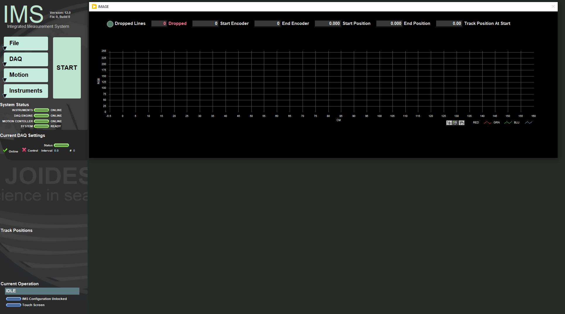
Figure 2. IMS Control window (left) and Instrument' windows (right).
The IMS Control panel (Figure 3): Provides access to utilities/editors via drop-down menus.
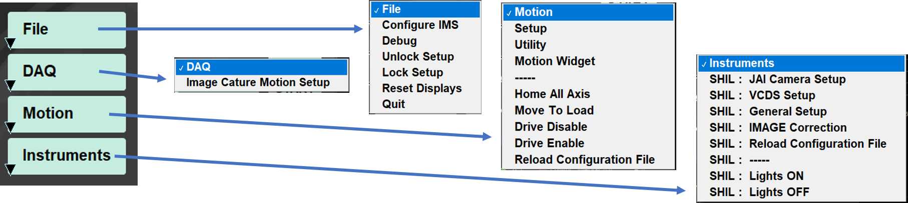
Figure 3. Control Panel Drop Down menus.
START button will allow the user to begin measurements. Section Information window (Figure 4) will pop up.
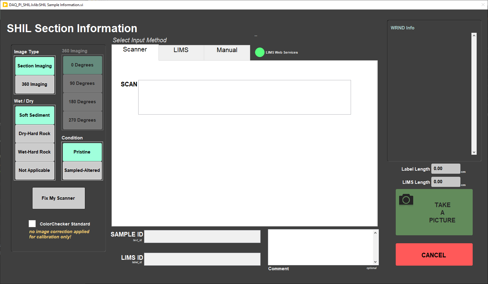
Figure 4. Section Information window.
B. Camera Setup and Calibration
The laboratory technician calibrates the system when needed by adjusting camera settings and analyzing an imaged Xrite Color Checker Mini standard (MacBeth card). Be sure to use a 2014 or newer version of the Xrite Color checker because the RGB values used for correction uses the values from the newer standard. The RGB values on the standard are calculated from the L*ab values provided by Xrite. As of we are using RGB values calculated under an illuminant A. The excel spreadsheet of RGB values of the Xrite color checker using varying illuminants and can be found here. The white square has R=240, G=242, B=235 and the black square R=50, G=50, B=50. A 3-D standard that holds the Xrite color checker and a grey silicon mat is in the SHIL calibration drawer, PP-2B (Figure 5).
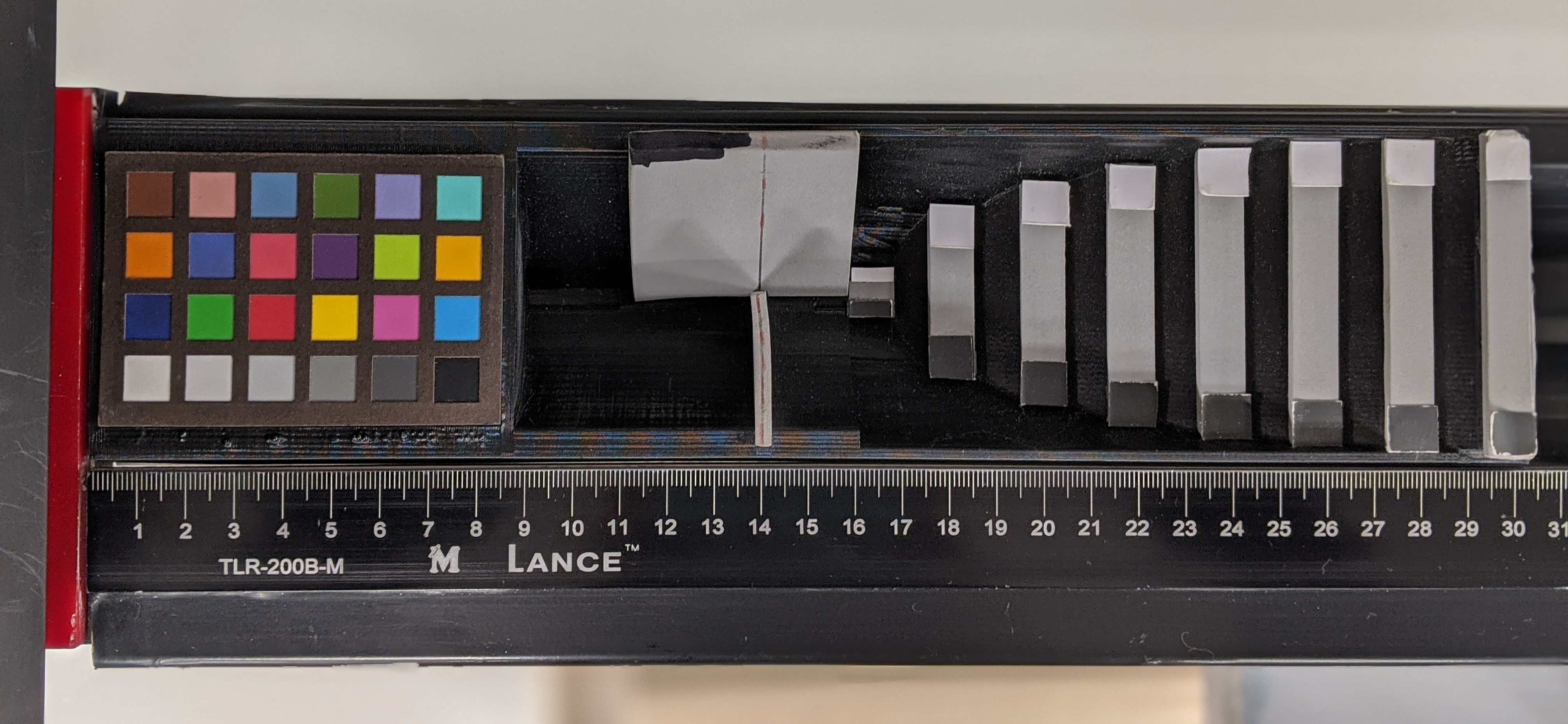 Figure 5. 3D standard with Xrite color checker standard.
The current light system (Figure 6) obtains nearly uniform illumination intensity from the core’s surface (half or whole round) to the bottom of the liner by a combination of high intensity, overlapping large diameter light source, close coupling to the imaged surface and the “line” image plane. The bottom edge of the led mount should be set between 2 and 4cm from the image surface. Note, any height change to the lights requires re-calibration. Heat is removed from the LEDs and transferred to the surrounding air via the copper heat pipes and is cooled with mini fans. While the copper rods can get hot they are not a burn hazard. However they are very delicate and bend at the slightest touch, so use care when working with the camera lens. For more detailed information on the theory behind the calibration please refer to the Understanding the SHIL Calibration for further reading. Maintain temperature of the lights at 30-40 °C during calibration. LED's of temperature is located above the camera. During a section scan the temperature ranges between 30-36 °C.
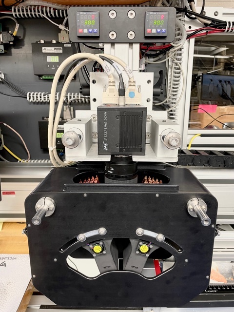
Figure 6. SHIL Camera and Lights set up.
Calibration is conducted in the following steps.
- Physically set the camera at the correct height and focus. See Camera Height and Focusing.
- Set the saturation range for each channel of the CCD while maintaining the white balance between these channels for neutral colors (white, greys and black). See Setting Exposures and Setting Gains.
- Correct for uneven lighting, dark noise and pixel flatness. See Pixel Black, Shading and Flat Corrections.
- Calibrate and create a correction LUT for each RGB channel. See Image Calibration.
The first three steps are done using the JAI Camera Setup Utility, the 4th step is done using Image Correction Utility. Before opening the utility you must disable Motion Control so that you can move the camera by hand.
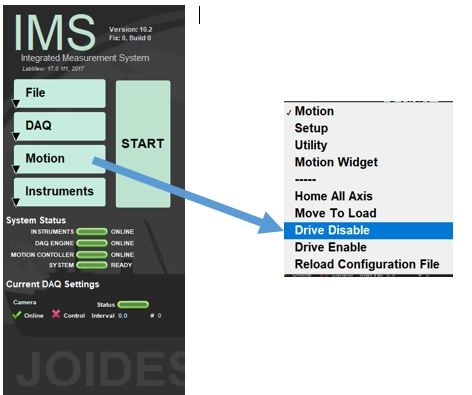
Disable Drive:
1. In the IMS control panel select Motion and then Drive Disable from the dropdown menu (Figure 7). You will have to move the camera by hand for the calibration, disabling the motor allows manual movement of the camera on the track.
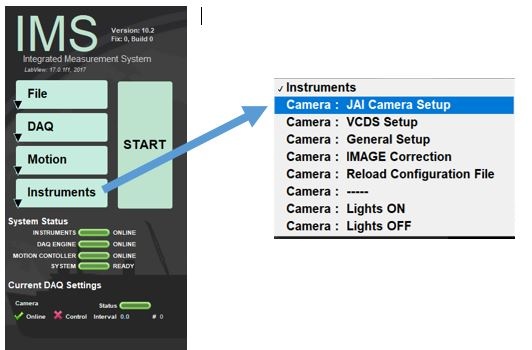
2. Open JAI Camera Setup utility: In the IMS control panel click Instruments > JAI Camera Settings (Figure 8). The lights turn on automatically when the JAI Camera Setup window opens.
Camera Height and Focusing
Camera Height
In practice the camera height rarely changes and this step is not necessary to perform for every calibration but it should be checked at the beginning of each expedition.
The goal is to set the across image pixel pitch with a focused camera. Warning this can be tedious and requires two people.
1. Turn on the lights. Remember to maintain temperature of the lights at 30-40 °C.
2. Click the START GRAB button.
3. Move the camera so that it is scanning just the centimeter marks on the QP 101 card (Figure 10). Also, it is important that the QP 101 card is mounted straight so that the scale lines are parallel to the direction of motion.
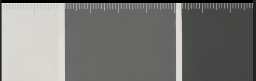
Figure 10. QP 101 card showing centimeter marks for pixel pitch calibration.
4. On the screen you will see the cm lines and vertical peaks on the Profile graph (Figure 11).
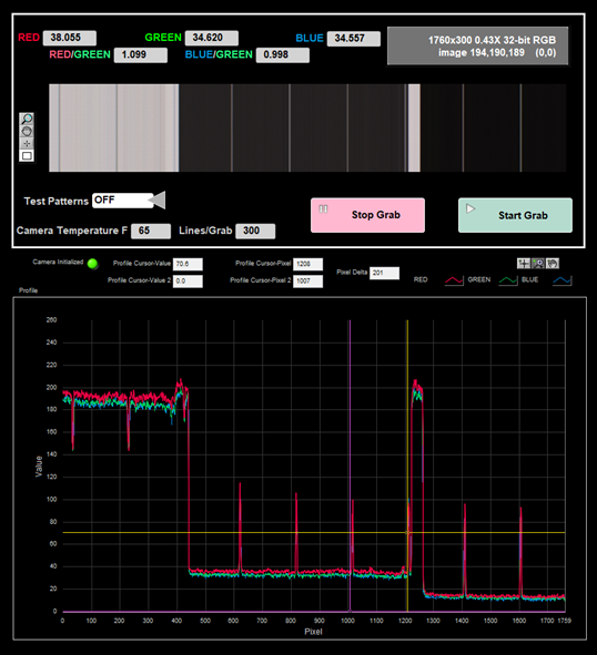
Figure 11. Example of the QP-101 marks and the profile graph.
5. On the Profile graph, drag the purple and yellow cursors to the center of two adjacent peaks near the center of the image. These peaks are the centimeter lines in the QP card.
6. Use the graph controls and expand (zoom) the graph horizontally (Figure 12).
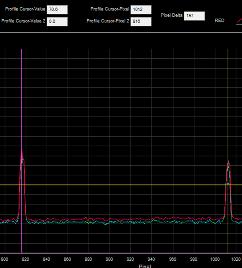
Figure 12. Cursor placement on the QP 101's centimeter marks in Profile graph.
7. In the expanded view, adjust the cursors so that the are centered in the peak's width (not necessarily the max value). You want to achieve a Pixel Delta of 200 pixels/cm (+/-1px) (Figure 13).
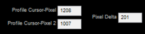
Figure 13. Cursor pixel values and span.
A word of caution.
Be careful how you tighten the clamps holding the camera to the T-Slot. Make sure to tighten with even pressure on both sides, if you don't the camera can be offset and you will see the image in the Grab window shift. The camera attachment method is not ideal and should be replace.
After performing this process you need to check the home position. When at the home position, the camera should be scanning the edge of the tray where the section is placed against (red strip). If not, you will need to adjust the home switch on the track until it does. An improperly set home switch will affect the placement of the crop window and potentially the offsets assigned to the RGB values.
Setting Exposures
1. Click the Gains-Black-Shade-Flat tab (Figure 14).
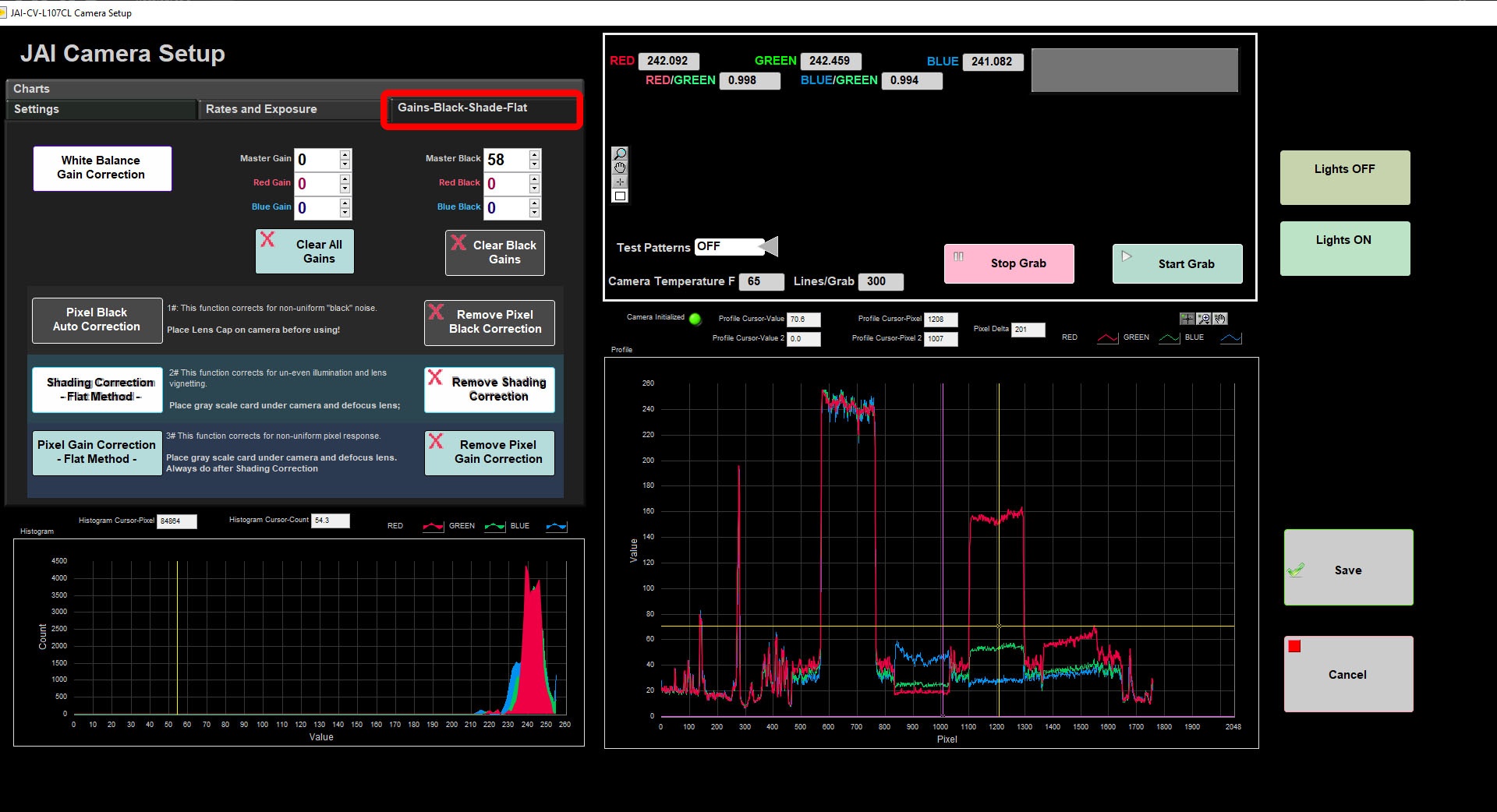
Figure 14. JAI Camera Setup Window showing the Gains-Black-Shade-Flat tab. The Gains-Black-Shade-Flat tab is outlined in red.
2. Click the Clear All Gains, Clear Black Gains, Remove Pixel Black Correction, Remove Shading Correction, and Remove Pixel Gain Correction (Figure 15). You will notice all values in the Master and Black gains go to zero.
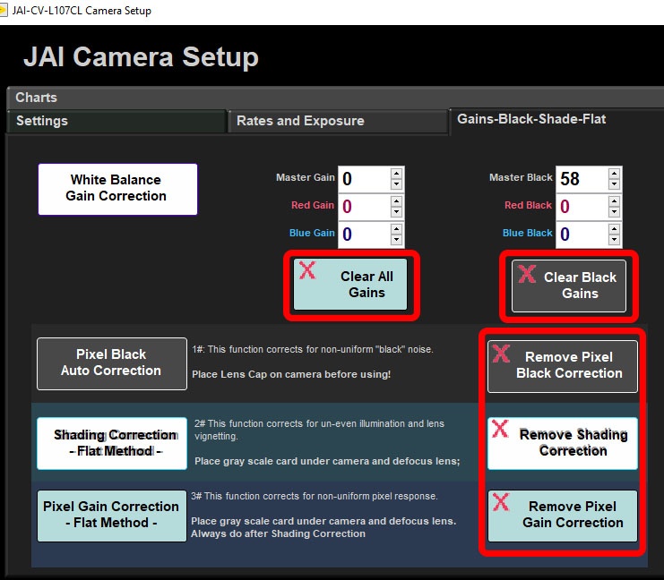
Figure 15. Remove the corrections and clear gains.
3. Check the camera's f/stop which should either f/16 or f/22 (see Figure 16). Remember that the higher the f-stop the greater the depth of focus. The down side is that a higher f-stops means less light and low light levels mean longer exposures - which means slow track speeds for scanning - which could impact core flow in the lab. So on a low recovery expedition you can afford the longer scan time, so go for f/22 otherwise f/16. If you are doing 360-imaging f/22 is a must. Check with the LO and EPM if you are unsure of the time needed for scanning sections.

Figure 16. Setting the F Stop on the Camera. Although the figure says f/22 is recommended (recommended by the manufacturer) onboard we found f/16 works best for our scanning needs.
4. Place the 3D Calibration Standard in the track. The color square must be oriented as shown in Figure 17.
Figure 17. Calibration 3D standard with the Xrite color checker mini.
Understand Triggers and Exposures
When the camera moves it will receive trigger pulses from the linear encoder. Each trigger pulse will start an exposure in the cycle. The encoder will provide 200 pulses for every centimeter of movement; therefore, the speed of the track controls the time between pulse which controls the maximum allowable exposure period. The individual exposure periods for the RGB channels must be completed in this time or lines will be dropped.
When setting up the JAI camera we are not moving and not receiving trigger pulses. In this mode we use the line rate trigger (free run) to simulate the encoder trigger period.
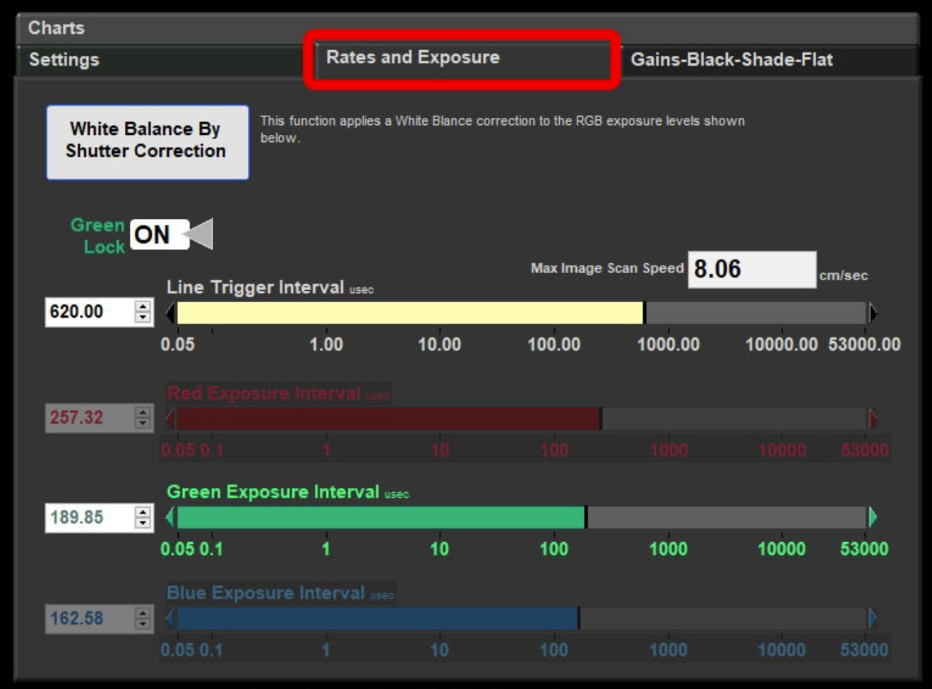
When you adjust the Line Trigger Interval (yellow slider in above figure) you will notice that the Max Image Scan Speed value changes. If you scan faster than this, you will drop lines but you can scan slower without affecting the calibration.
You can adjust scan speed in the Image Scan Setup window as well (figure below). When you click Save in the Image Scan Setup window the value will be updated. The Speed in the Image Scan Setup should always be lower, not higher, than the Max Image Scan Speed calculated by the Line Trigger Interval. As a general rule we want to stay at 8 cm/s or higher value to maintain core flow in the lab.

After you done a few calibrations you will develop a feel for what is possible with current camera set up but if you are just starting we recommend setting the line rate to emulate a scan speed of 8 cm/s.
CHANGING EXPOSURE VALUES
Now you are ready to start setting the exposures for the RGB channels.
1. Turn on the lights.
2. Click the START GRAB button (Figure 18).
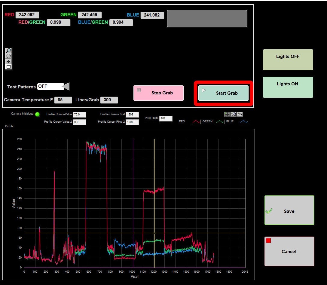
Figure 18. Start Grab.
3. Move the camera over the White square on the Xrite Color Checker standard.
4. Use the mouse and draw a ROI (Region of Interest) with only the white square inside (Figure 19). The RGB values and Ratio values will only be calculated for the pixels inside the ROI (Figure 20). Place the cursor in the white square, right-click and draw a rectangle by dragging diagonally. Release the mouse when you have selected most of the white bar. The rectangle (marked in green) should only have the white color and nothing else inside.
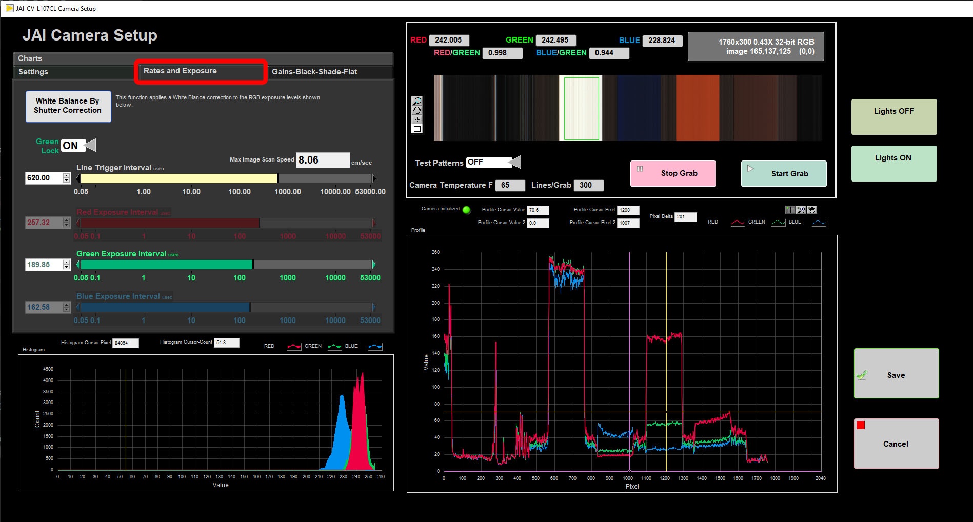
Figure 19. Selecting the ROI of the White square.
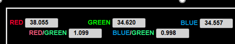
Figure 20. RGB and Ratio values calculated from the pixels in the ROI.
5. Go to the Gains-Black-Shades-Flat tab and click the Clear All Gains and click Clear Black Gains if not already done.
6. Go to the Rates and Exposure tab and set the Green Lock to Off. That step allows you to adjust the exposure intervals (Figure 21).
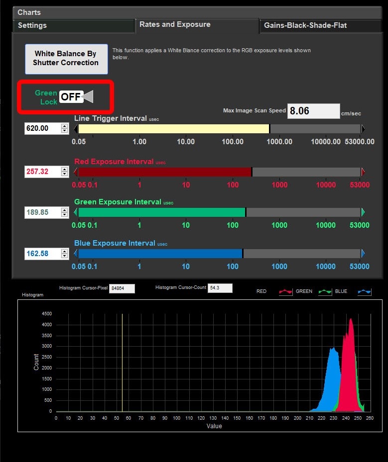
Figure 21. Set Green Lock off.
Weakest RGB Channel
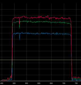
It is helpful to know which RGB channel has the lowest intensity because this channel will be the limiting factor when setting exposures. To find which channel is the weakest remove all gains and set identical exposure values for the RGB channels. The intensities will look like the figure below. Onboard our weakest channel is Blue.
7. Start with the blue channel (the weakest channel), increase the Exposure Interval time until Blue value is near 240.
8. Adjust the green exposure interval until the blue/green ratio is near 1.000 (+/-0.005).
9. Adjust the red exposure interval until the red/green ratio is near 1.000 (+/-0.005).
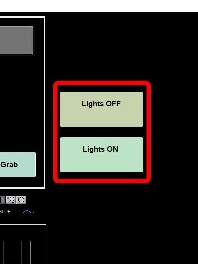
10. Click Lights Off. Once you have initially roughed in the RGB channels for the White Color Checker square, it is time to look at the black (dark) corrections.
Note: The Line Trigger Value must be greater than the Exposure Intervals for Red, Green, and Blue.
If you cannot get the blue channel to 240, you have several correction options:
1) Lower the lights for increased illumination.
2) Open up the f-stop for more light.
3) Increase the line rate (slower scan speeds) so that you can increase the exposure period.
4) Use gains to amplify the signals.
Using gains to amplify the signal is the simplest choice because the other options are not practical or desirable. The down side of using gains is that they amplify both signal and electrical noise. Amplifying noise is not good so use gains sparingly. In the next section we discuss how to use the gains but remember you will likely move back forth between setting exposures and gains to optimize the camera. It is an iterative process.
Neutral Balance - is the Xrite color checker neutrally balanced?
Note that the RGB values for the White square are R=240, G=242 and B=235 for the 2019 Xrite color checker standard. Thus the ratios for B/G and R/G are not 1.000 (as we describe to achieve in steps 8 and 9 above).
B/G = 0.97, R/G = 0.99 (Xrite color checker v. 2019)
Previous color standards used onboard had balanced RGB values, meaning the R, G and B were equal, hence achieving B/G and R/G rations of near 1.000 was the goal. With the 2019 Xrite color checker these values are not balanced for white so achieving 1.000 may not be the ideal ratio for color balancing.
What ratio is best to use needs to be tested. It may not make any difference, but when time allows we should test update this User Guide if any difference is found in the calibration curve.
Setting Gains
What are gains?
What is the difference between regular gain and the black gains? Think in terms of a linear calibration where the regular gain sets the slope (multiple) and black gain sets the offset (addition). So changes in the the regular gain value will have little affect on dark colors but changes in the black gain will offset all colors equally. The gains labeled "Master" are applied to all channels while the red and blue apply corrections to only those channels.
White Balance via Master Gain Correction
1. Open the Gains-Black-Shades-Flat tab (Figure 22).
2. Increase the Master Gain until the the Blue value is near 240.
3. If the other Red and Green values are too high as a result of increasing the Master Gain, you can apply negative gains to those channel until the R/G and B/G ratios are back to near 1.000 or you can re-adjust the exposures. Re-adjusting the exposures is preferred.
Once you have initially roughed in the RGB channels for the White Color Checker square, it is time to look at the black (dark) corrections.
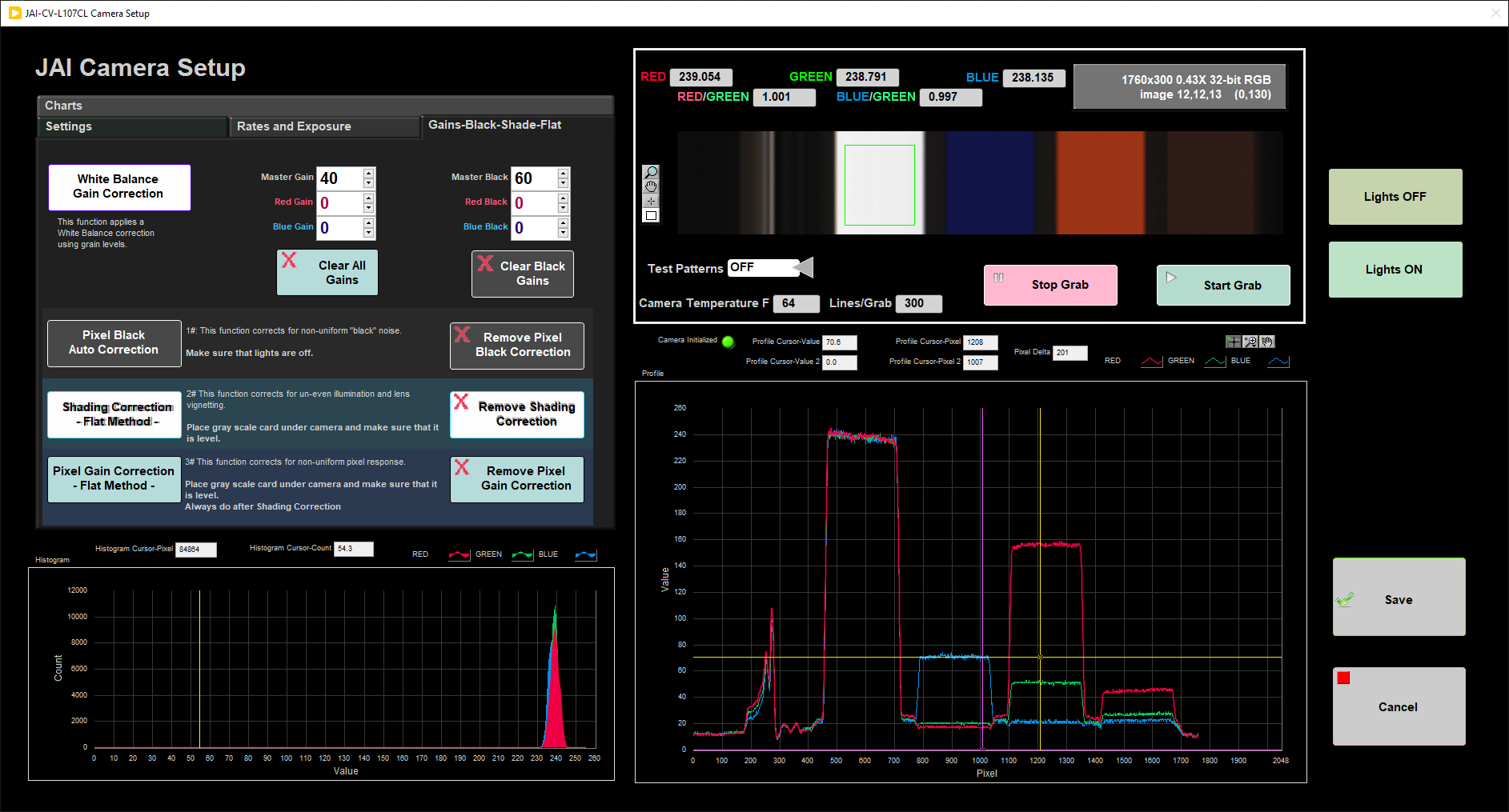
Figure 22. Adjusting Master Gain to bring the Blue values up to 240.
Setting the Black (Dark) Values
1. Turn on the lights.
2. Click the START GRAB button.
3. Move the camera over the black square on the ColorChecker standard.
4. Use the mouse and draw a ROI (Region of Interest) with only the black square inside. The RGB values and Ratio values will only be calculated for the pixels inside the ROI (Figure 23).
5. Adjust the Master Black value unit the Green value is near 15. 40 is a good starting value for and we increasing to 60 works best.
6. Adjust the Red Black and Blue Black Gains until the ratio are close to 1.000 +/- 0.05. The RGB values of the Black square is balanced (R=50, G=50, B=50) so achieving a ratio of 1.000 is best.
Keep an eye on the histogram graph on the bottom left corner (Figure 23). We want all the colors to overlay each other pretty closely. Adjusting the RedGain and BlueGain will move the colors (histograms) in the graph in the lower left, move until they are over lapping.
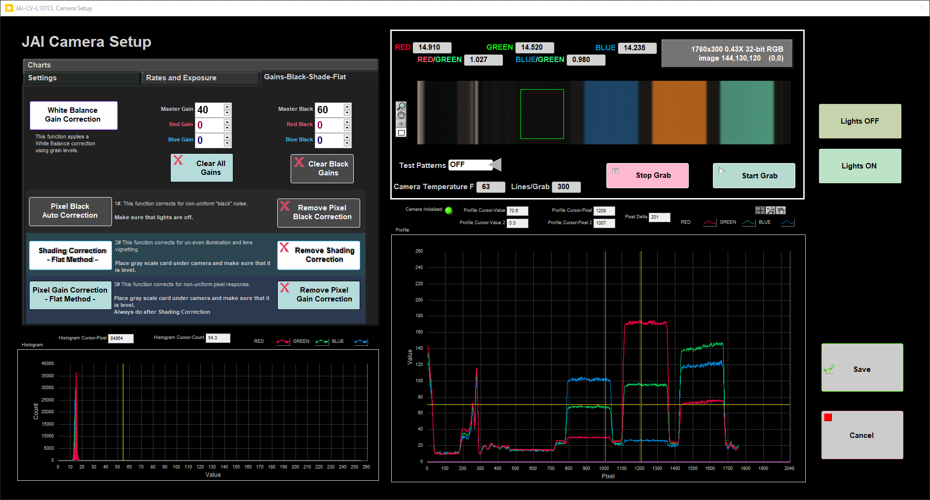
Figure 23. Adjusting Master Black, RedBlack and BlueBlack to reach RGB values of 15 for black square.
Adjusting gains likely changed the RGB values in the White square of the Xrite Color checker. Move the camera back over the white square. Draw an ROI box in the white square. If the values aren't near 240 go back to the Rates and Exposure tab and adjust the the gains values. Check back in the Black square and see its still about 15. Adjust the gains and/or exposure intervals until the Black RGBs read near 15 and White RGBs read near 240. This is a balancing act and can be tedious. Remember do not let the temperature to go about 39°C white doing the balancing.
The Problem with Black
The issue with black is that there is very little energy at this level and noise makes up a significant % of the value. The next issue is that the cameras response from bright to dark objects is non-linear. The ColorChecker value is actually near 50 but do not try to obtain that value by jacking up the gain. It just doesn't work! By convention we aim for RGB values of ~15.
Getting a white balance is also difficult. Once you set the green to 15 move the camera so that you view the color just above the black and use the red and blue black gains to get a good white balance.
Pixel Black, Shading and Flat Corrections
We apply three corrections Pixel Black, Shading and Pixel Flat (gain). Only do the corrections after you have finished the first "rough in" adjustment of the RGB exposure and gains. Obtain the heat resistant silicone gray mat from the drawer PP-2B. The heat resistant silicon mat is homogenous in color which is helpful for the corrections (no mottling as seen in the old grey cardboard card).
Pixel Black Auto Correction: The pixel black level represents extra energy (dark noise) in the camera independent of a light source and is a consistent pattern in the sensor. To correct for this the light source must be turned off and the camera internal correction circuit collects a few lines of data. An average is taken across the line, and pixels are either added to or subtracted from in order for each pixel to have the average value. (Vendor Manual Reference)
Shading Correction - Flat Method: Shading effects can come from an uneven distribution of light and along the outer edge of the camera lens. Shading is corrected for by averaging the signal across a group of eight pixels to represent the line.
Pixel Gain Correction - Flat Method: Each pixel has a different response to a fixed light source. To correct for this non-uniformity a couple lines of data are calculated and the average response of the pixels are calculated. Then each pixel has a correction factor applied to bring all pixels to the average level. The Pixel Gain Correction also corrects for some shading effects and should be done after the shading correction.
Image Streaking
Image striking is caused when used a non-uniform standard for the Pixel Gain Correction correction or just from dirt. Until we found the silicone sheets we would have to defocus the lens to mitigate this issues. If see streaks chack your target material and repeat this correction.
Pixel Black Auto Correction
1. The new light set up makes adding a lens cap difficult so it has been decided and tested that the pixel black auto correction can be done without the cap. But Ensure the lights are off.
2. With lights off click Pixel Black Auto Correction. The RGB lines in the Profile graph should be uniform (Figure 24).
![]()
Figure 24. Pixel Black Correction applied.
Shading Correction
- Take the heat resistant gray silicone mat and wooden board from the SHIL calibration drawer. Clean off any dust with a piece of tape (Figure 25). Dust will cause unwanted artifacts in the image. The mat must be clean and flat on the track.
- Place the heat resistant gray silicone mat on the track. Make sure that it is level and perpendicular to the camera’s axis.
- Click Lights On, and move the camera over the gray mat.
- Note for Tech: previously we defocused the lens to preform the Shading correction. That is no longer needed because the silicone mat is even in color/texture.
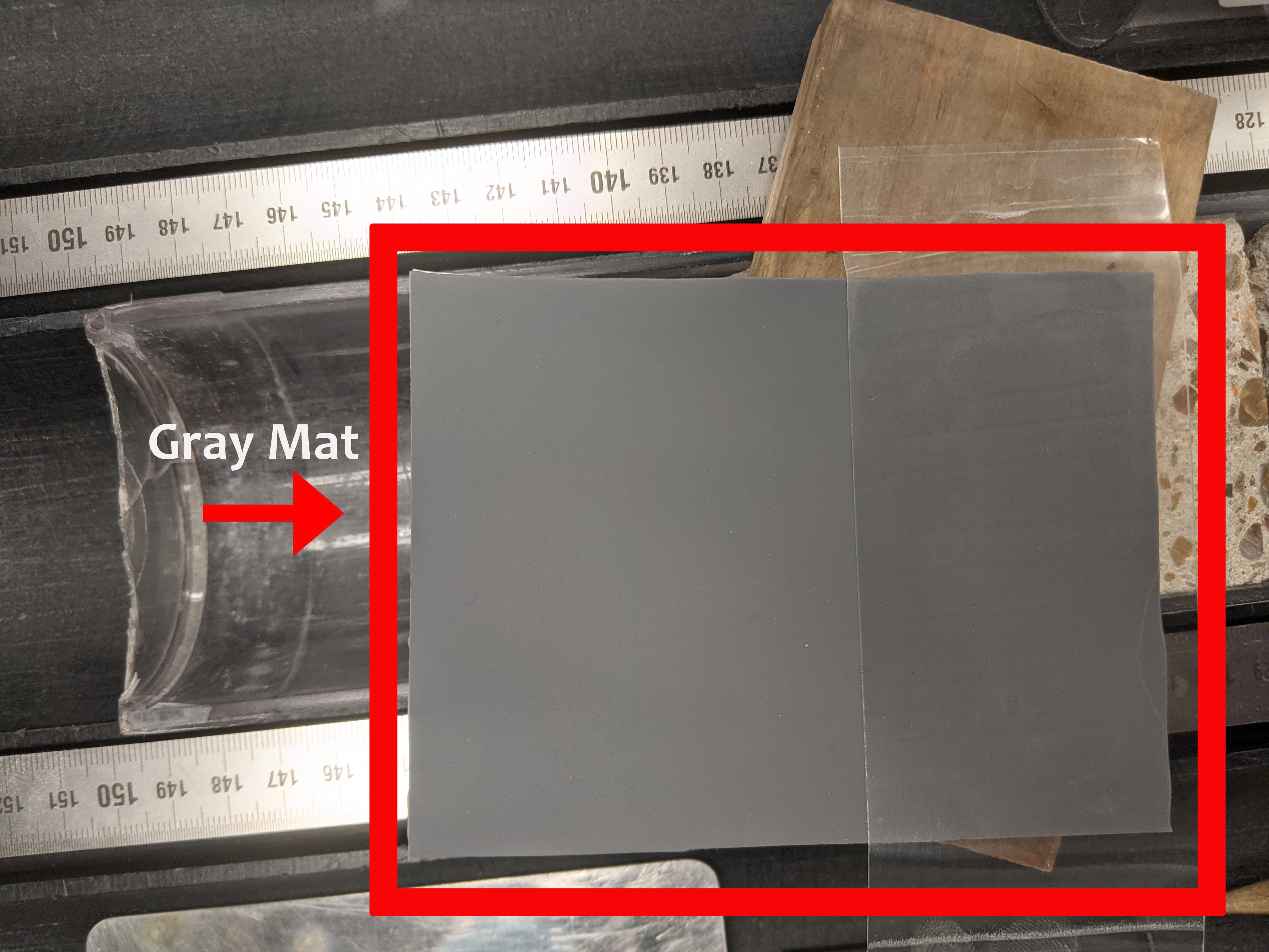 Figure 25. The Gray silicone mat being cleaned with tape.
5. The RGB lines should first appear “bowed” evenly across profile and centered in the image (Figure 26). If not check the orientation of the gray mat, it needs to be flat and perpendicular to the camera. This very important. A wooden holder was designed to hold the mat, it should be in the SHIL calibration drawer.
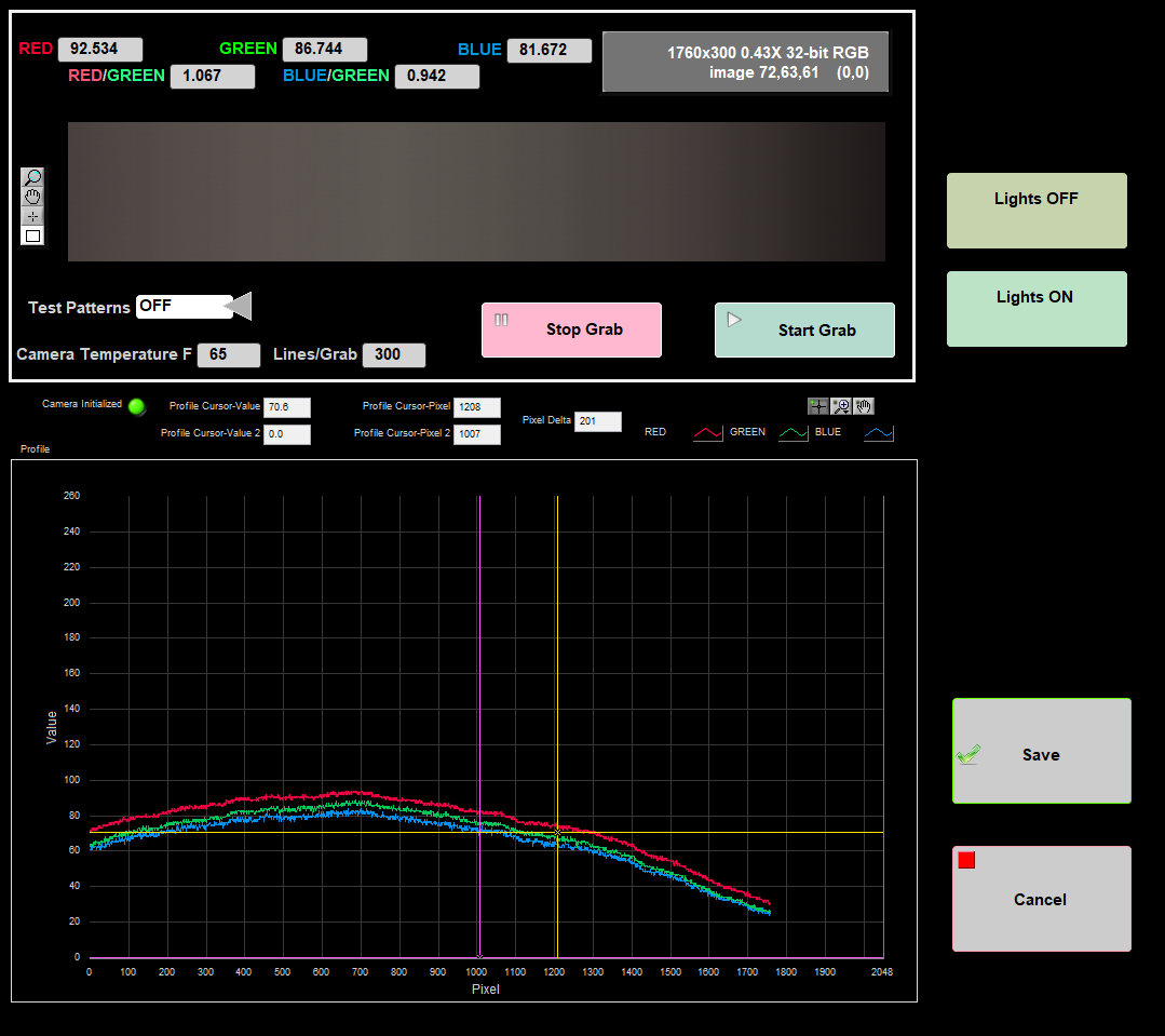
Figure 26. Grayscale card corresponding RGB Profile visible.
6. Click the Shading Correction - Flat Method button. This can take a few seconds, don’t click anything else until it is done. The RGB lines should now be flat (Figure 27).
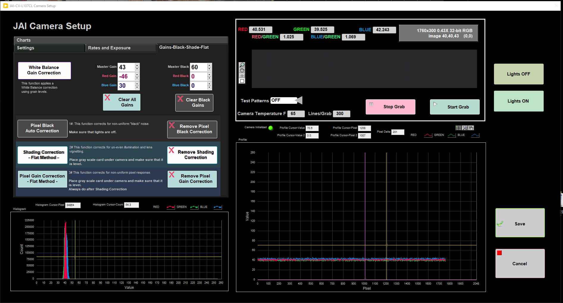
Figure 27. Image grab and profile after the Shading Correction has been applied.
Pixel Gain Correction
1. Make sure gray silicone mat is flat.
2. Click Lights ON
3. Click the Pixel Gain Correction - Flat Method button and move the camera slowly back and forth. This averages the pixels and helps eliminate streaking in the image. This will take several seconds, don’t click anything else until it is done. When its done the RGB lines should still be flat and the individual RGB the same, but may not be equal to each other.
IMAGE Calibration (Correction)
Before we can begin the calibration process, an uncorrected image of ColorChecker standard must be taken.
1. Place the 3D calibration standard on track as shown (Figure 28). Be sure to use the XRite Color checker 2019. The color squares must be oriented as pictured below, butted against the red reflection bar.
Figure 28. Color standard in track in correct orientation.
2. Open IMS and Click Start.
3. Scan the STND Color barcode label (Figure 39b). Check the ColorChecker Standard box (Figure 29a). With this box selected no corrections are applied to the image so we are able to assess the raw image quality.
4. Click Take A Picture.
5. When the image has finished click Crop and then Save. We use the uncropped tif image so the crop here is not important.
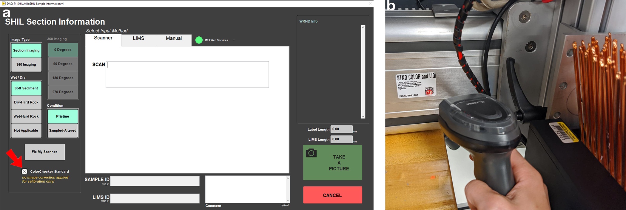
Figure 29. a) sample information screen with ColorChecker box checked, b) standard barcode being scanned.
6. On the main IMS panel select Instruments and Camera: Image Correction (Figure 30).
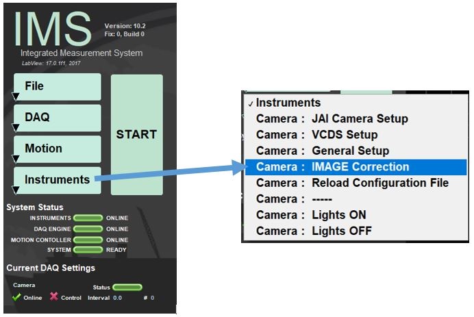
Figure 30. Image Correction command selection.
The main Image Correction window displays three main areas (Figure 31):
A. Graph panel: Main graphical viewing area on the left side of the screen.
Uncorrected Image Tab: Shows the measured red, green, and blue values of the gray scale color squares.
Applied Corrections Tab: Applies polynomial fit corrections to the RGB lines.
Compare: Shows a visual and RGB values of the Original color square before corrections, the Xrite Color checker standard and of the color after corrections are applied.
B. Image Viewing Panels: Area in upper right portion of the screen that displays the original and corrected test image and Xrite color checker.
Original: Displays the uploaded tiff.
Corrected: Displays the uploaded tiff with corrections applied.
Color Checker: Displays the known values of the Xrite Color Checker.
C. Correction Panel: Panel in the lower right portion of the screen that allows user to apply corrections to the image
TIFF Correction: Shows tiff red, green, and blue polynomial fit.
JPEG Correction: Shows brightness, contrast, and gamma settings.
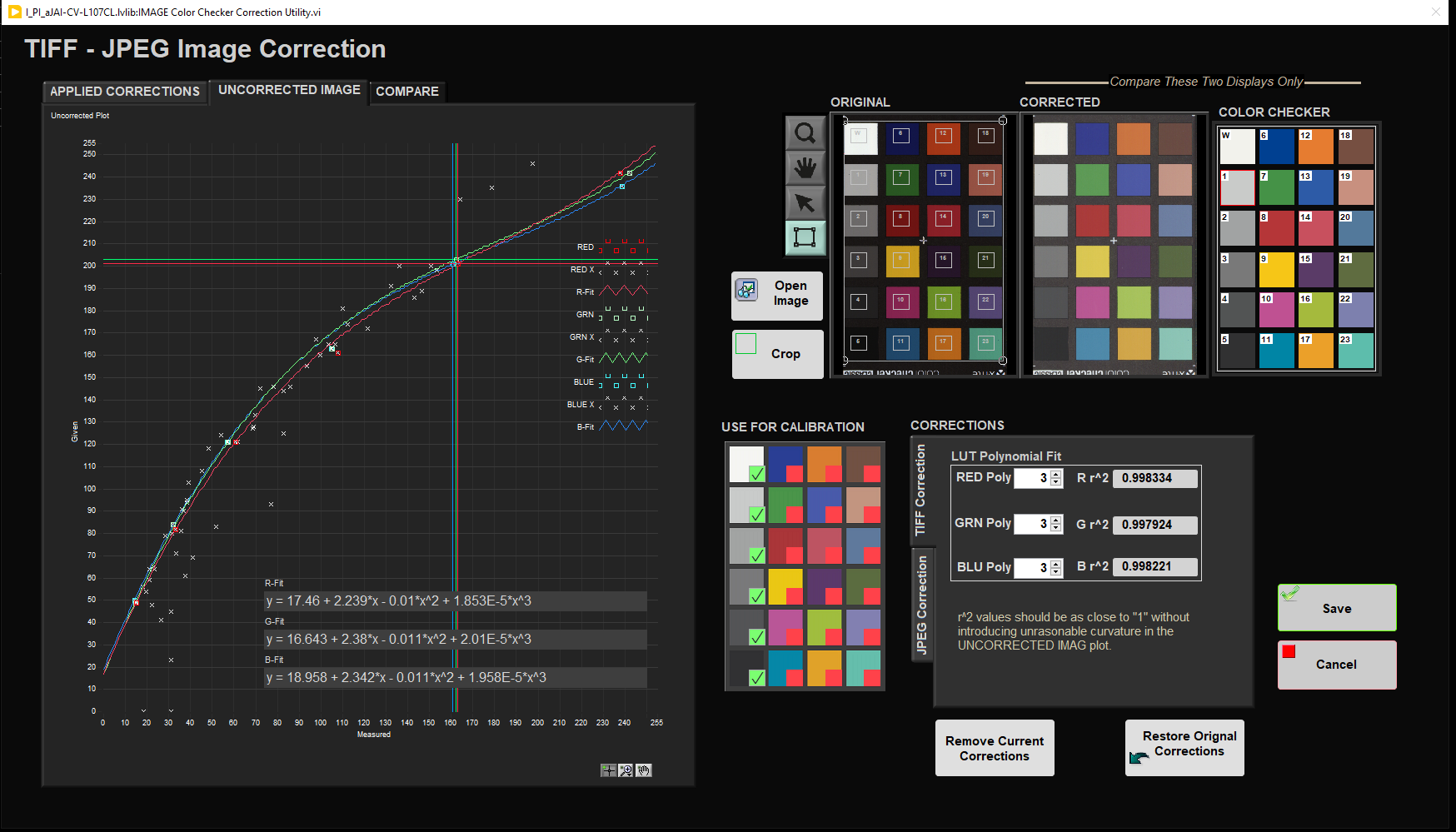
Figure 31: Image Correction user interface.
7. On opening of the Image correction window the program prompts you to select the TIFF file of the color standard you took. The image loads into both the Original and Corrected windows.
8. Draw a ROI box loosely around the color checker in the Original box (Figure 32-1)
9. Click Crop (Figure 32-2).
10. Draw another ROI box around the Color Checker squares and this time making sure to only have XRite color checker in the box. White squares will appear inside each square. Adjust the box to get those white squares close to the center of the color squares. Do not click Crop again.
11. Click the colors you want to use for the correction curve (Figure 32-3). As of use only the white, shades of grey and the black.
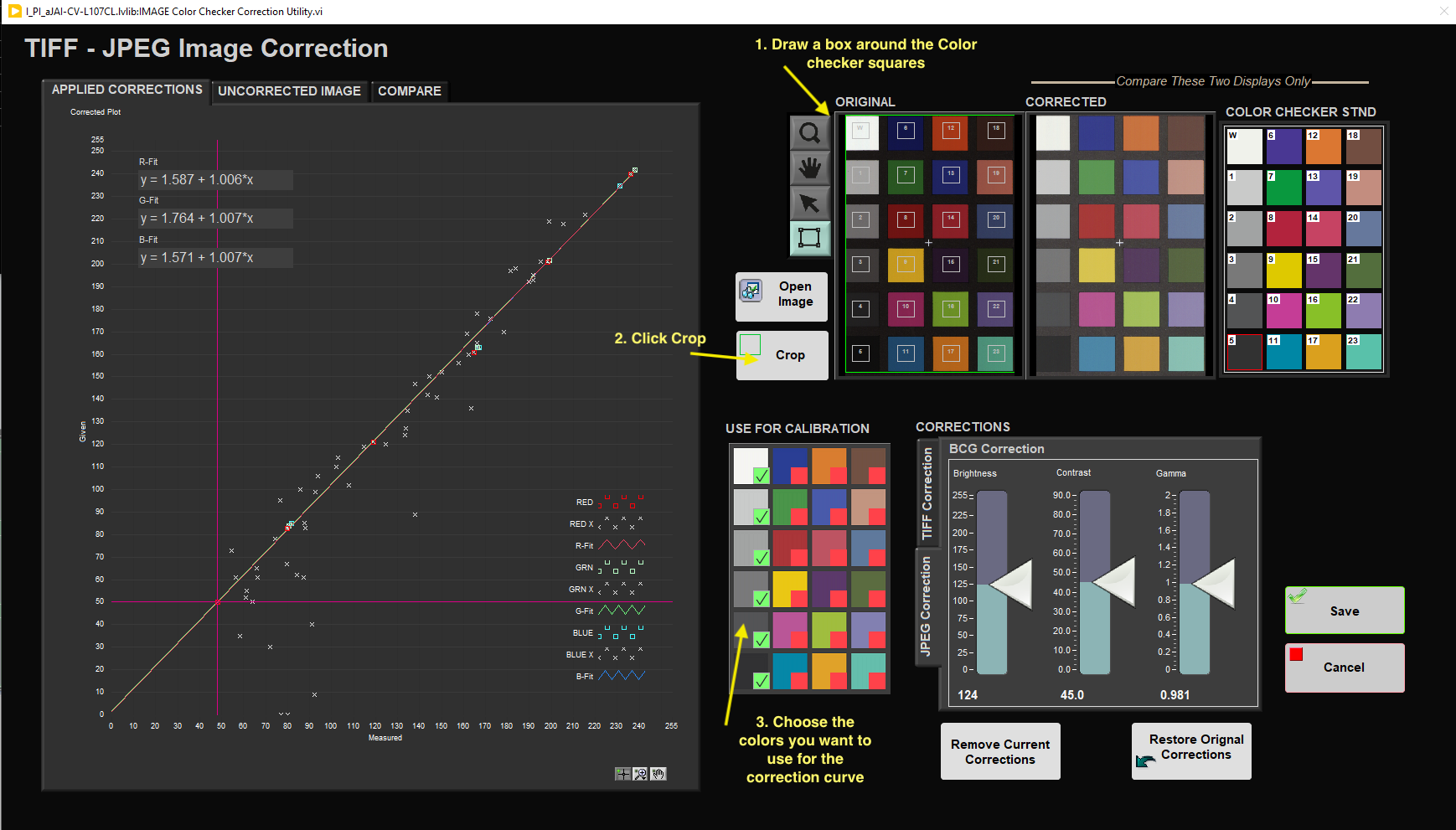
Figure 32. Image Correction Window.
Check TIFF and JPEG Corrections
Here we check and adjust, if needed, our TIFF and JPEG Corrections. You may find you only need to slightly tweak the values and the calibration is good. With the new lights we have found that no adjustments have been needed. However if the image appears streaky, a physical change has happened to the Camera or lights, the RGB values between corrected and expected are far off (>5), or the graphs of either the tiff or jpeg don't look good, you will need to re-calibrate following the full calibration discussed below.
TIFF Correction Check
1. Click TIFF Correction tab (Figure 33-1).
2. Click Uncorrected Image tab. This graph shows the measured red, green, and blue values of the color squares.
3. In the Tiff Correction tab adjust the LUT polynomial order values for the Red, Green, and Blue channels (Figure 33-1). Adjust these values to create the lowest residual error with the smoothest curve in the Uncorrected Image tab. Polynomial values should be about 3. Make sure that the curve does not wave about too much. If it does, the values need to be lowered.
4. In the Compare tab check that the corrected color square and Xrite color checker RGB values are very close (Figure 34). Make sure that the white does not exceed the Xrite values (RGB = 240, 242, 235). There is also a visual display so you can see the difference in color for the color checker and the corrected. If you are unable to produce a reasonable correction curve, it is necessary to redo your white balance correction described in the Calibration section below.
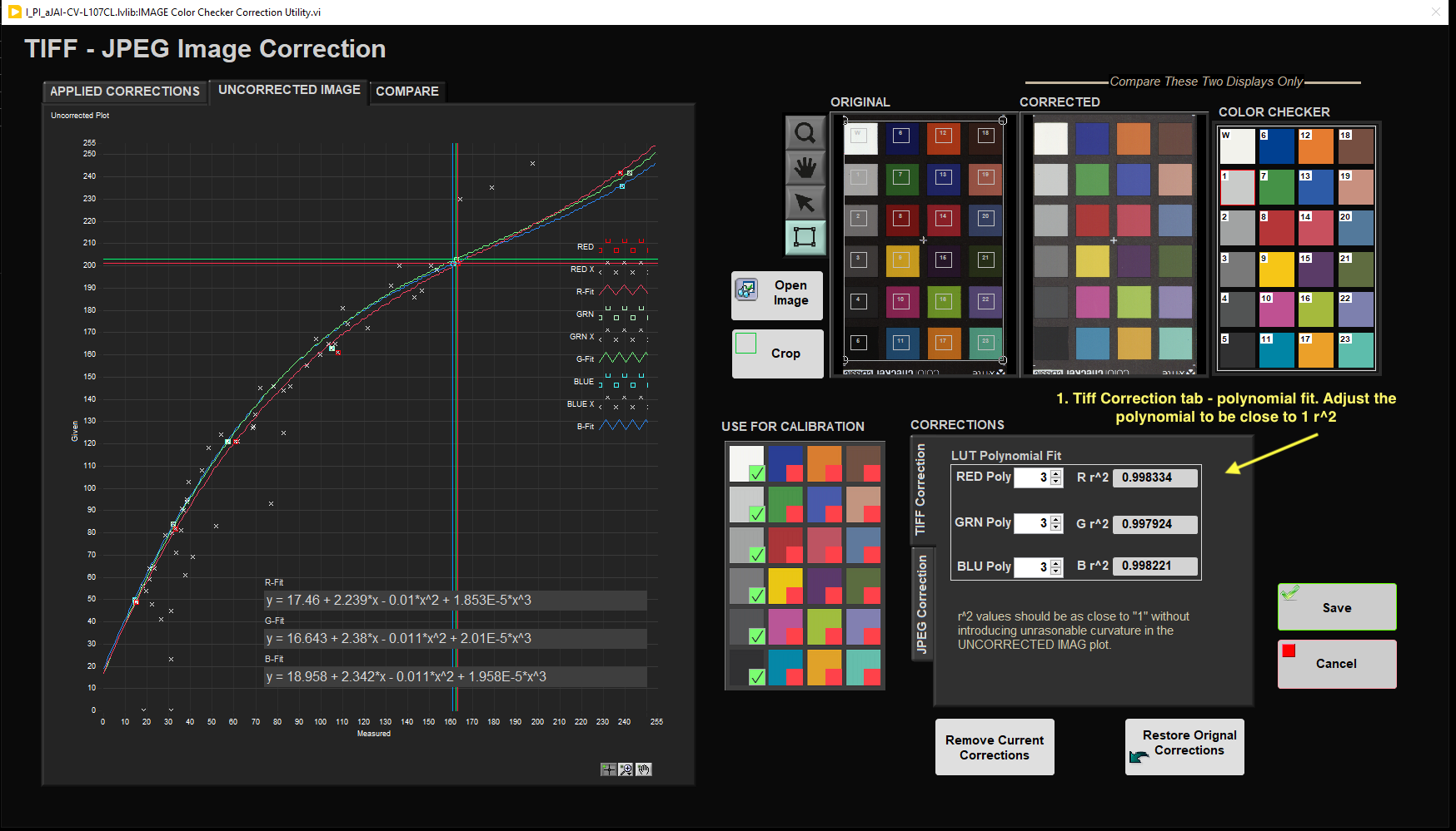
Figure 33. Tiff Correction
Note: the TIFF correction is applied to both the TIFF and JPEG image but for the JPEG image you can also apply a Brightness, Contrast and Gamma (BCG) correction (See JPEG Correction section below). This is done at the photographer’s discretion. With better balanced LEDs on the new light system you may not have to use the BCG corrections (leave the values at their mid-points. Figure 34).
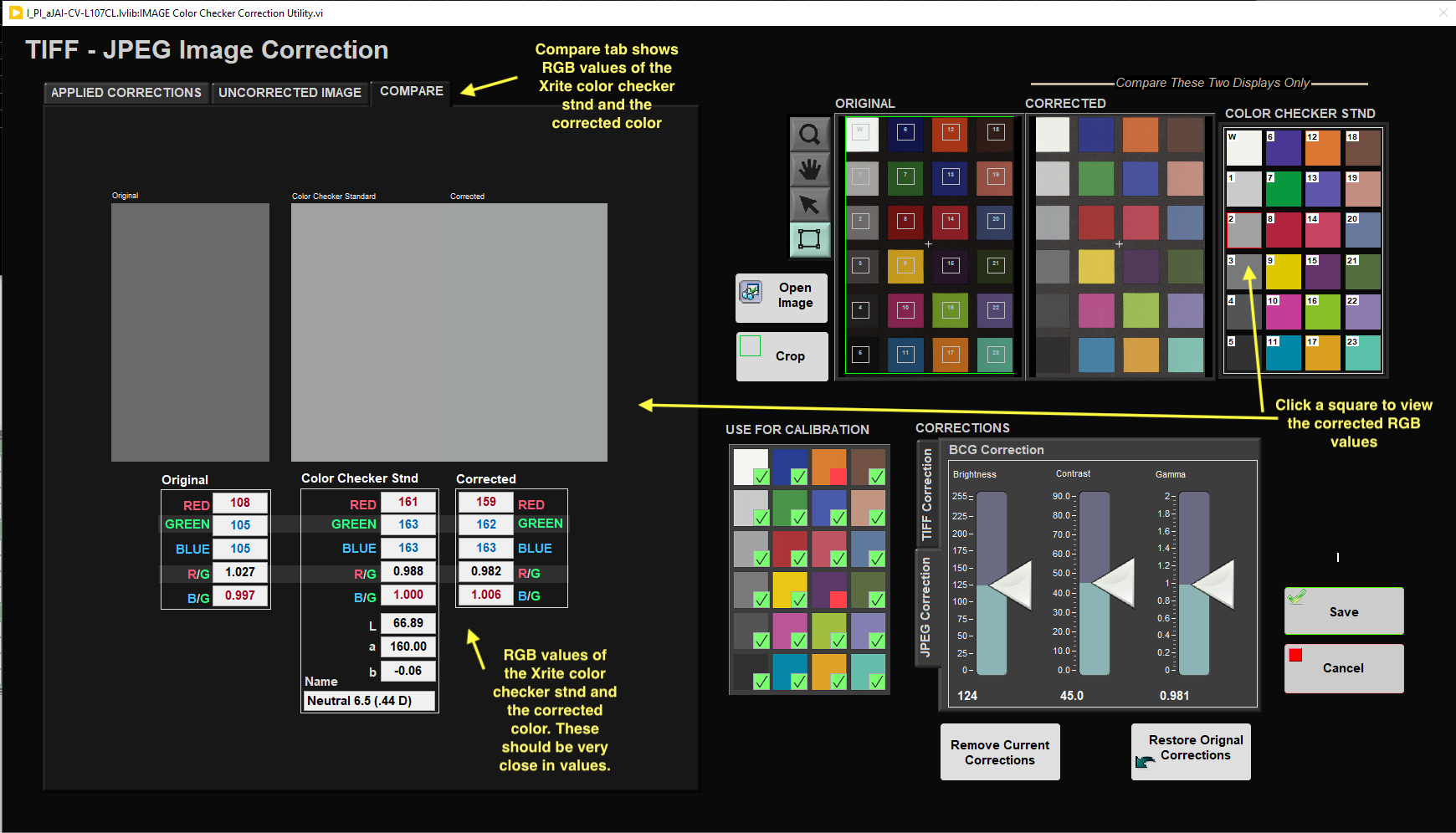
Figure 34. Use the Compare tab to view the RGB values for the Xrite color checker and the corrected.
JPEG Correction Check
In JPEG correction you will check and adjust, if necessary, the brightness, contrast and gamma (BCG) of the image. Situations may also arise where a JPEG correction should be applied. In the instance of very white or very dark cores, the TIFF images may look good but the JPEG images may look washed out or too dark to view details. JPEG corrections do not alter TIFF image settings. As mentioned above, with the new lights the BCG values may not need to be adjusted and to be kept at the mid values (Figure 35).
1. Click JPEG Correction tab (Figure 35-1)
2. Adjust the Brightness, Contrast, and Gamma levels (Figure 35-1) to achieve a straight line in the Applied Corrections tab and the RGB Corrected values in the Compare tab should have values near 242 for the white square and near 50 for the black. We want a linear relationship between the measured and given values. Each BCG setting adjusts the line in different ways and there are many different ways to adjust the values to achieve a linear relationship. You want to achieve a good image with good brightness, where the image has good saturation and not too washed out. The Applied Corrections Graph should be a straight line and the ROI Corrected box for the color selected (Figure 35-2, 35-3) should have values near the RGB values of the Color Checker STND. These may change depending on the instance of extreme colors, extremely white or extremely dark cores, in which the settings may have be tweaked more to get a user friendly consumer image.
3. If the values are good and there are no streaking issues in the images or other unwanted artifacts, you can click Save and no further adjustments are needed. However if you have determined the doesn't look good, click Cancel and you can proceed to the following Calibration section and complete the calibration instructions listed.
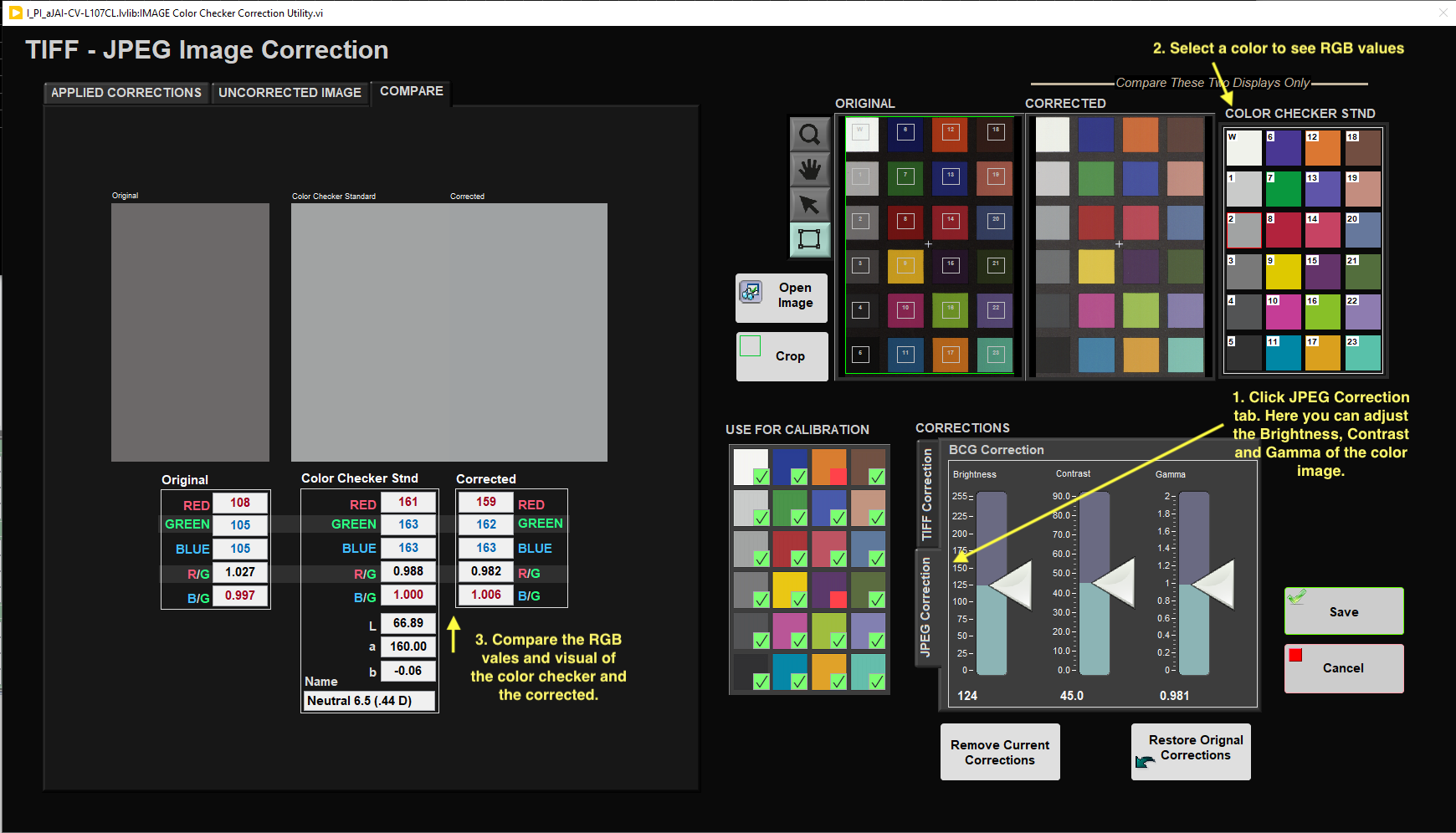
Figure 35. JPEG Correction using Brightness, Contrast and Gamma.
Image Check on Calibrated Monitor
Check the final scan:
1. To double check your calibration under the same scanning conditions as the scientists see, scan an image of the 3D standard without the color checker box selected.
2. Click Crop and Click Save
3. Copy the image to a shared network folder to view on a calibrated computer screen in the Imaging Office. Images located in the C:/DATA/IN/IMAGE folder.
4. Open the TIFF and JPEG in Photoshop in the Imaging Office (calibrated computer).
5. Visually examine each file you just preformed to ensure the colors, neutrals, mid-tone and contrast are true to the real values, and that the scan is free from artifacts. Use the eyedropper tool in photoshop to see the values of pixels (Fig. ## Figure needs to be added).
C. Set Measurement Parameters
a) Instrument Setup
- DAQ > Image Capture Motion Setup (Figure 36)
Figure 36. Image Scan Setup window
2. Instruments > Camera: General Setup (Figure 37).
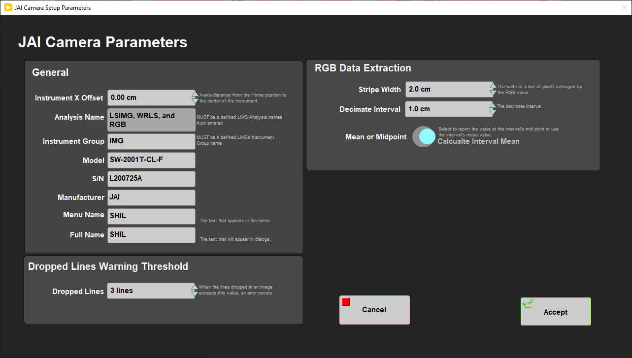
Figure 37. General Camera Setup window
3. Instruments > Camera: JAI Camera Setup (Figure 38).
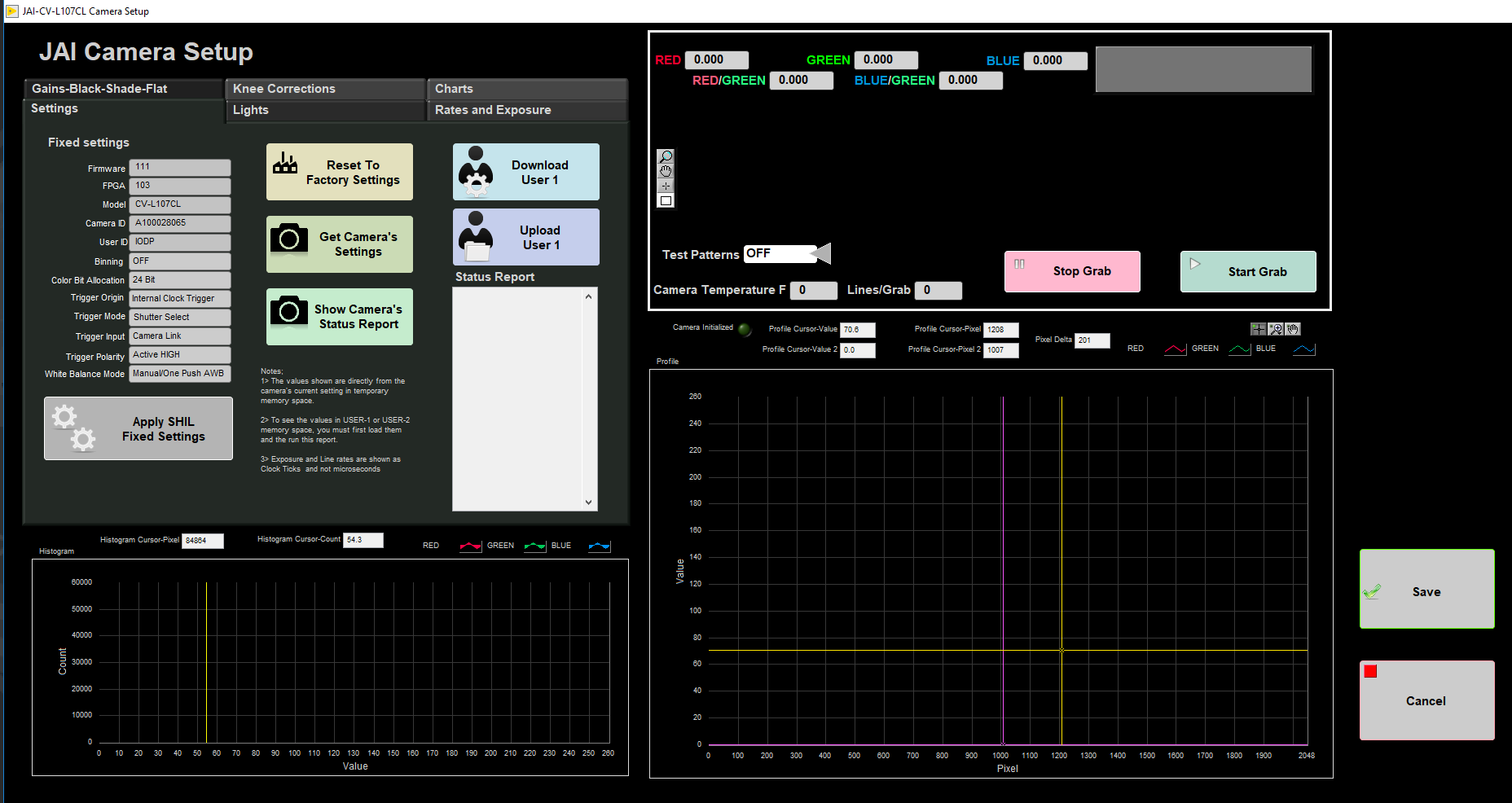
Figure 38. General Camera Setup fixed Settings
b) Set Measurement Parameters
Adjust measurement parameters before beginning measurements. Users can adjust the RGB settings and camera speed.
RGB
Users can adjust three RGB parameters: decimate interval, stripe width, and whether to use the mean or midpoint RGB value. For more information regarding how RGB data is calculated please see Appendix A: RGB Calculation. Two RGB files are automatically created after each image is saved, a high resolution RGB file and a lower resolution decimated RGB file. Both files are uploaded to LIMS and can be found in the expanded report on LORE. The high resolution RGB files are produced with default values and can not be modified. The resolution of the lower resolution RGB file can be set by the user as described below.
Adjust RGB Settings
1.Go to Instruments > Camera: General Setup (Figure 39). The JAI Camera Setup Parameters window will appear (Figure 39).
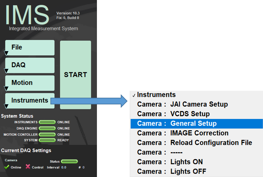
Figure 39. Select JAI Camera Setup Parameters window
2. Adjust values in the 'RGB Data' setting controls (Figure 40).
- Stripe Width: Centered in the middle of the core, this determines the width across the core that will be used to calculate RGB data. This is typically set to 2cm. While the value can be changed higher or lower it is commonly at 2 cm. The advantage is this width provides enough material to not exaggerate small disturbances but rather provides RGB data representative of the bulk lithology.
- Decimate Interval: The interval that sets the recorded offset along the length of the core. This value can be set between 1 - 2.9 cm
- Mean or Midpoint: Can choose how RGB is calculated for the interval. Interval mean calculates the mean RGB values over the interval. Interval Midpoint uses the RGB value at the center of the interval. This is typically set to Interval Mean.
Figure 40. JAI Camera Setup Parameters window
The 'General' and 'Dropped Lines Warning Threshold' should not need to be adjusted. If something needs to be altered talk to the programmers and ALOs.
3. Click 'Accept' to save values. If select 'Cancel' the values will revert back to prior settings and the window will close.
Camera Speed
Camera Speed is calculated during the calibration procedure. The camera speed set must be lower than the speed determined by the calibration or else the camera will start 'dropping lines'. Dropped lines means the camera is moving too quickly to calculate the RGB and offsets at the bottom of the core will return values of '0'.
Adjust Camera Speed
- Go to DAQ > Image Capture Motion Setup (Figure 41).
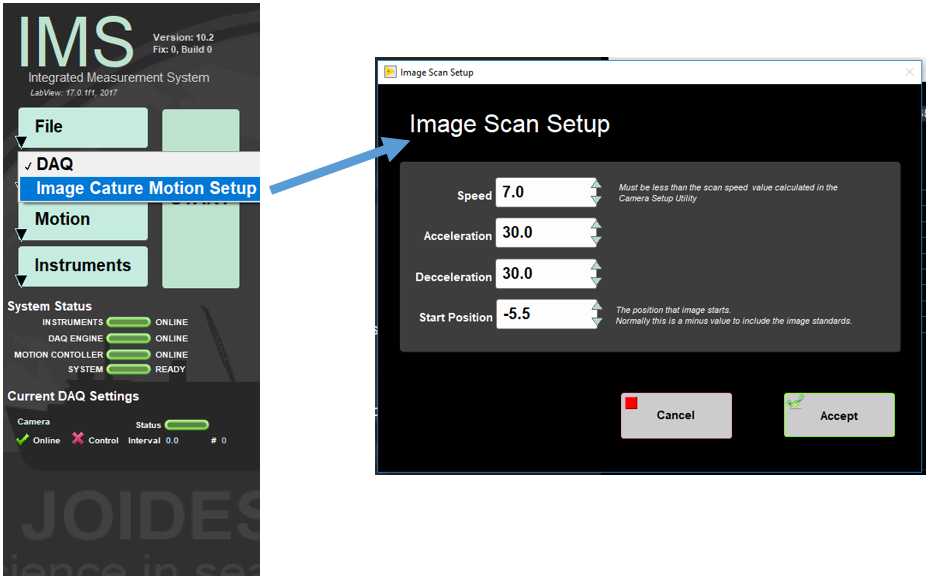
Figure 41. Select Image Scan Setup window
2. The Image Scan Setup window appears. There are four settings in this window:
- Speed: This is the speed in cm/sec the camera moves while measuring the section. This speed must be set lower or equal to the speed determined by the Camera Calibration.
- Acceleration: The rate in cm/sec the camera ramps up to when not measuring a section.
- Deccelaration: The rate in cm/sec the camera will slow down when not measuring a section.
- Start Position: This is the position the imaging begins. Note it will be a negative number. The top of the core starts at 0 cm in order to image the standard gray-scale card in front of the core, that location will be negative.
D. Preparing Sections
Sediment
The surface of the archive half generally needs to be scraped after splitting to clean the sections and better reveal layering and structures. Sediment cores should be imaged as soon as possible after splitting and scraping are completed to minimize color change through oxidation and drying.
Hard Rock
Rock pieces should be dry and individually rotated such that the split face is approximately perpendicular to the axis of the camera. The lights and lens aperture are configured to give consistent illumination and focus to effectively image rubble bins.
For 360 Imaging of hard rock cores refer to the section 360 Imaging Hard Rock.
Loading Section
- Pick up section half and place in the track loading area with the blue end cap forward against the color block. Make sure the section is pushed all the way against the block so the end cap is lined up with 0 cm on the ruler.
- Bring the endcap for the section to the SHIL workstation for entering sample information.
- If the section has a whole round sample taken, denoted by a yellow bottom endcap, place a split styrofoam spacer at the end of the section. Cut the styrofoam to same length of the sample taken and write letters on the styrofoam to indicate the type of the sample taken. For example a 5 cm Interstitial Water whole round sample taken. A 5 cm styrofoam spacer with 'IW' written on it would be placed at the bottom. Once a spacer has been made it can be used over the course of the expedition for applicable section halves.
E. Making a Measurement
NOTE: Before taking images make sure the lights and camera are set up and calibrated properly.
a) Sediment
1. Click the green Start button in the IMS Control panel (Figure 42).
2.The SHIL Section Information window will pop up.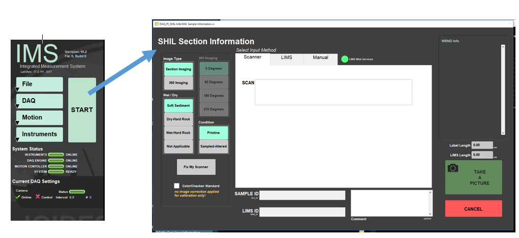
Figure 42. Select SHIL Section Information window
3. The area on the left has four fields to define the condition of the sample measurement:
- Image Type: 'Section Imaging' or '360 Imaging'. For instructions on the 360 imaging refer to 360 Imaging Hard Rock section.
- Wet/Dry: Indicates the type of the material being image
- Condition: 'Pristine' or 'Sampled-Altered'. Sampled-Altered could include imaging the working half or a highly disturbed section. Most instances should be Pristine.
- 360 Imaging: This area is grayed out unless '360 Imaging' Image Type is selected. For instructions on the 360 imaging refer to 360 Imaging Hard Rock section.
Select the conditions appropriate for the section half.
4. There are three ways to enter sample information into IMS (Figure 43):
- Barcode (most common): Put cursor in the 'Scan' box. Use the bar-code scanner to scan the label on the end-cap. The sample information will parse into the 'Sample ID', 'LIMS ID', and Length fields.
- LIMS Entry: Select the 'LIMS' tab at the top of the window. Navigate through the hierarchy to select the correct, expedition, site, hole, core, and section. Length information will automatically populate when the section is selected.
- Manual Entry: Select the 'Manual' tab at the top of the window. Click in the box and manually type sample information into the box.
By default the instrument is set for imaging the archive half and will not allow you to scan a working label. If you want to take a picture of a working half you need to go to the MANUAL tab and select W (working) into the Section Half label (Figure 43). Once you have selected W (working), you will not be able to scan an archive half; in order to do that you need to go back into the MANUAL tab and re-select A (archive).
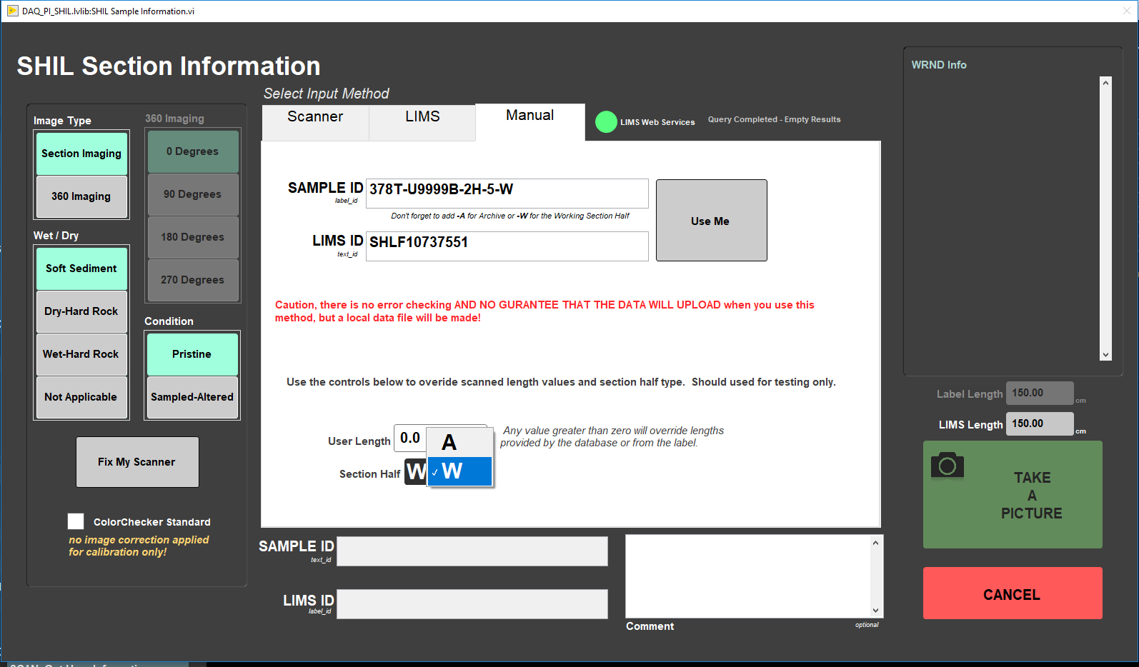
Figure 43. SHIL MANUAL Section Information window
5. Click Take a Picture. The lights will turn on and start moving down the length of the core. In the IMS interface the sample information will go away revealing the measurement windows. The image and RGB data is displayed and updates as the measurement progresses.
6. When the measurement is complete, the camera lights will turn off and move back to the home position on the track.
7. The Image Crop window (Figure 44) pops up. An image should be cropped to include all material and the inner edge of the end-cap. RGB data will exclude data outside of the Crop area. The green box is the IMS estimation of the crop area. Click and drag the green lines to adjust the cropped area at the top, bottom, and sides of the image. Tools in this window include:
- Show Bottom of Image: Takes image down to illustrate the bottom of the image and crop box.
- Show Top of Image: Brings image up to show the top of the image and crop box.
- Crop Image: Crops the image to show only image inside of the green box.
- Uncrop Image: Will undo a crop and allow user to re-adjust the green crop box.
- Save Image: Saves the image, RGB data, and writes the upload files
- Discard Image: Does not save the image or RGB data.
The Image crop restricts users to limit adjustments to 2cm or less. The message box will indicate if the crop has exceeded allowable limits and the 'WRND Info' message box indicates if and where any whole round samples were taken from the section. If the image needs to cropped by more than 2cm check the correct section/end cap is being uses, a styrofoam spacer is not missing, and the curated length. Cores can expand so if the curated length is incorrect, talk to the curator on shift to correct the length. Note this will also create a need for the curator to re-calcuate depth of the hole. If the error is in the curated length of the core a user can check the 'override crop restriction' button to crop the image and upload the data.
8. Click Crop Image when satisfied the green box will capture the entire image.
9. If satisfied with the image click Save Image. If the image needs to be re-imaged click 'Discard Image' and re-start the measuring process.
10. The 'Image CROP' window will go away and the 'SHIL Section Information' window will appear again.
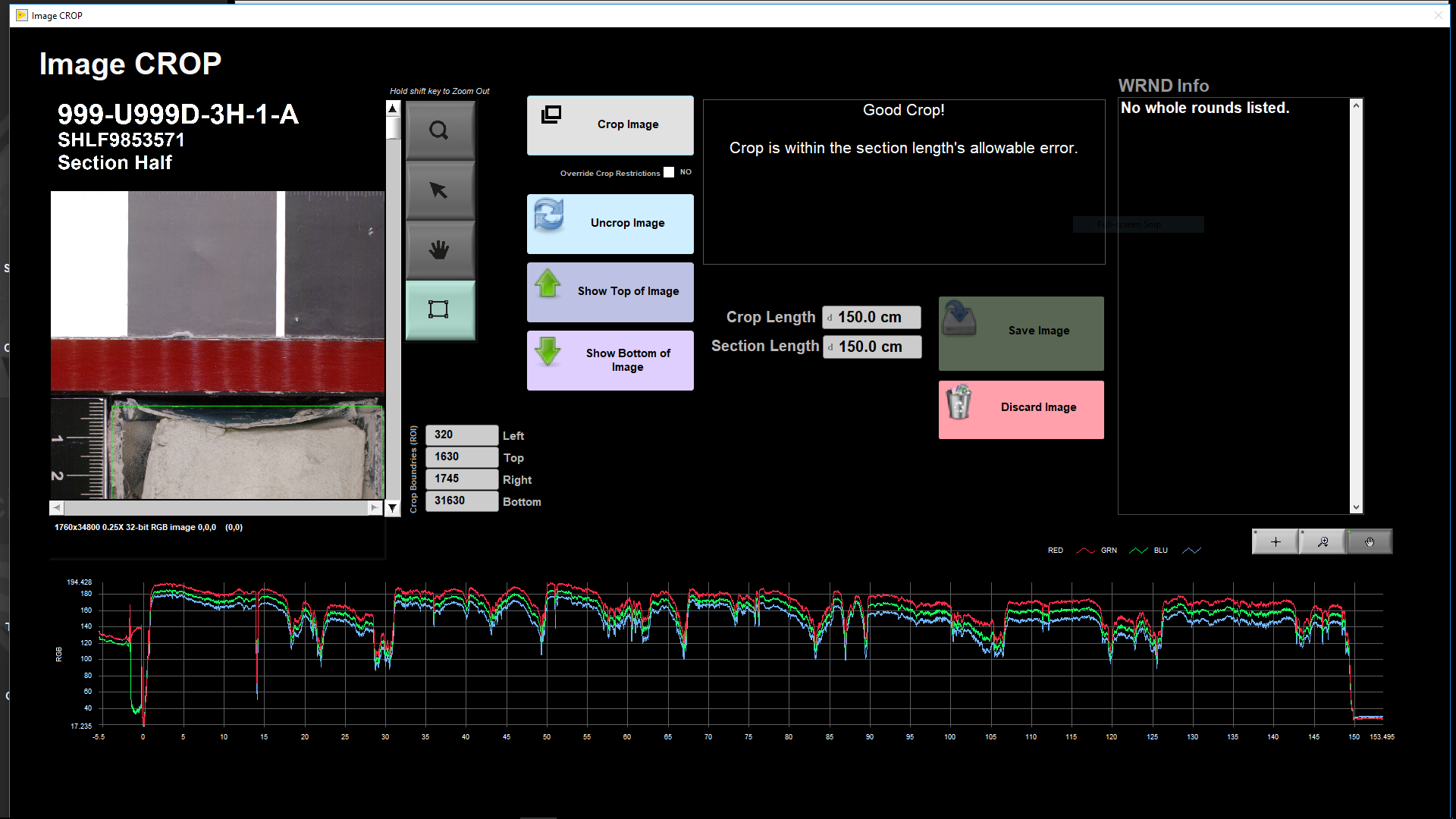
Figure 44. Image CROP window
b) 360 Imaging Hard Rock
The SHIL can be used to image the external surface of whole round hard rock cores in order to assemble a 360° composite image of the whole round. Oriented rock pieces are imaged after they have been binned and the structural scientist has marked the split lines on the pieces. Using the custom whole round scanning tray, the whole round core surface is imaged four times at the 0°, 90°, 180°, and 270° orientation from the splitting line. The Imaging Specialist will download the images and assemble a composite image from the four scans and upload the composite separately.
Sample Preparation
1. Remove the section half scanning tray from the SHIL and replace it with the whole round scanning tray making sure to align the blocks correctly. Note that the rotating section of the tray has 0°, 90°, 180°, and 270° markings on each end and that the rotating section will click and lock into each orientation.
2. Place the split liner section with the whole round core on the tray below the SHIL and align the top with the 0 cm on the ruler on the tray (Figure 45).
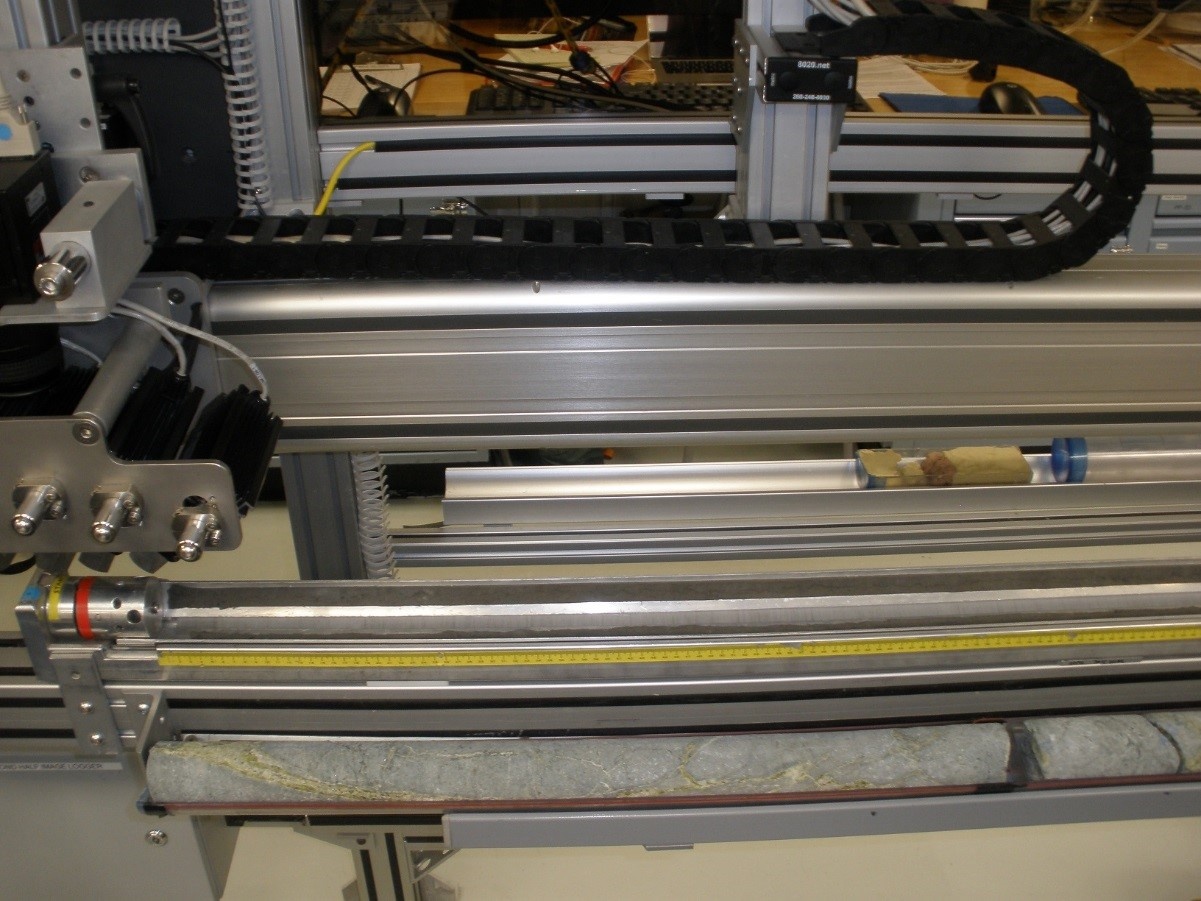
Figure 45. Whole round core correctly placed on the split liner section.
3. Remove the 0° aluminum strip and another aluminum strip on either side of 0°. Move the dry, oriented pieces into the tray, keeping the pieces at the correct offsets and aligning the split line with the 0° orientation.
4. Attach the not 0° aluminum strip and rotate the tray so that the 0° position is up, facing the camera (Figure 46).
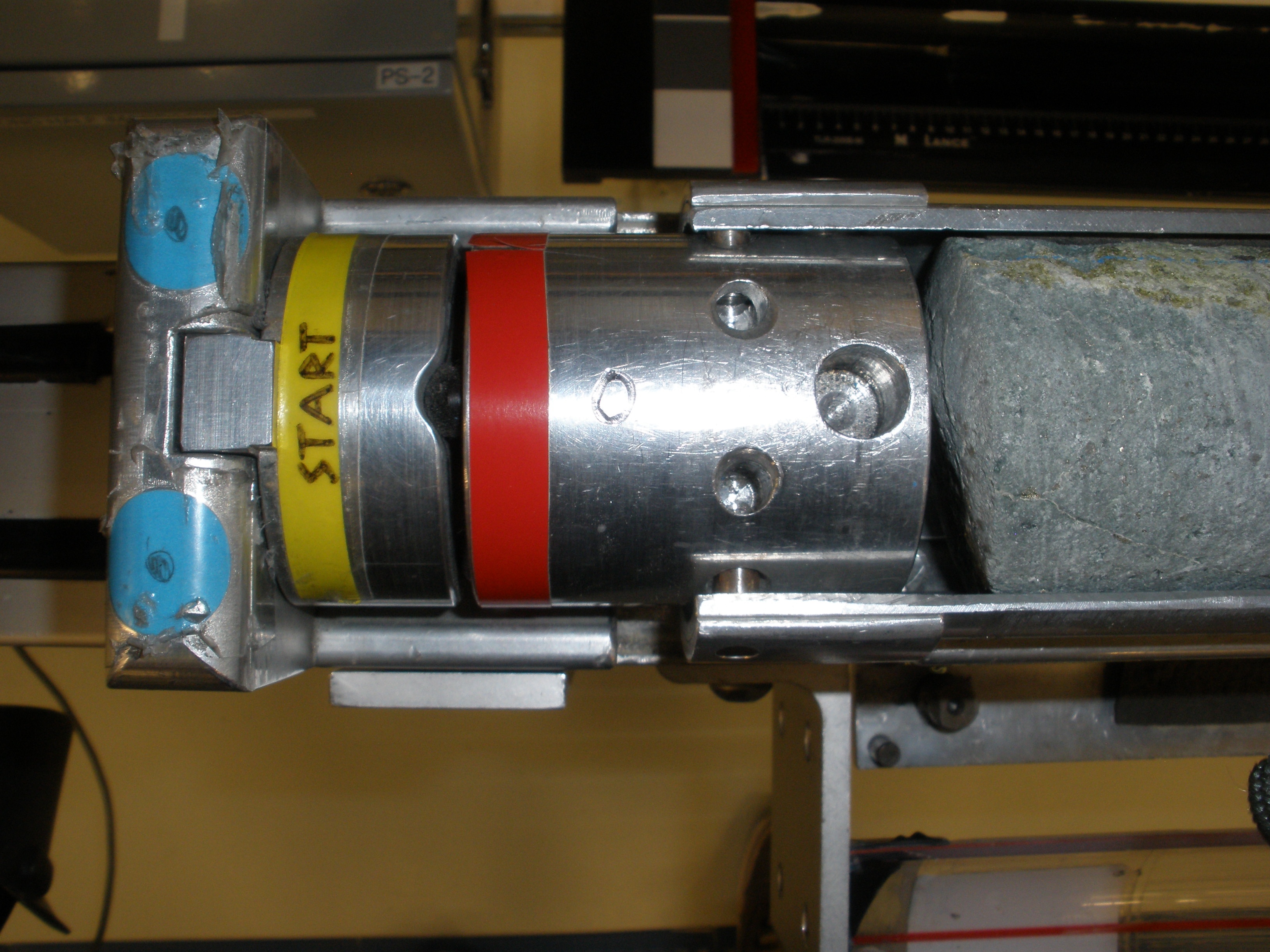
Figure 46. Whole round core correctly placed on the aluminum tray
Take Image
1. Click START and the SHIL Section Information screen will appear (Figure 47).
2. Scan the section barcode from the endcap
3. Select the 360 Imaging on Image Type and the default quadrant will be 0 Degrees. Select Dry-Hard Rock. Click TAKE A PICTURE
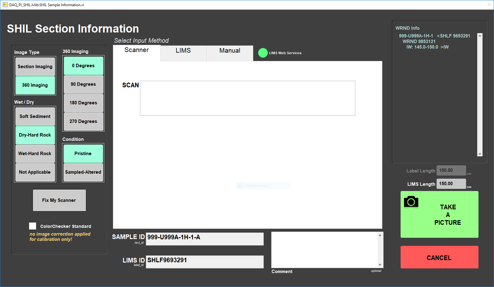
Figure 47. SHIL Section Information window for 360 Hard Rock Imaging
4. When the scan is finished, the Image CROP window will open. Crop the image and Save it.
5. The SHIL Section Information window for whole round will open and the rotation angle will default to the next quadrant, in this case 90 Degrees.
6. Replace the aluminum strip and rotate the tray to the next position, remove the aluminum strip facing up. Ensure that the rotation angle setting in the window is that same as on the tray. Click TAKE A PICTURE.
7. Continue the cropping, rotating and scanning process until all quadrants are complete. Once the images are uploaded to the database, the Imaging Specialist will create the 360 composite image and upload it to the database. If an image is discarded, the software returns to the main screen and the user will need to start a new 360 scan. However, the user can select which quadrant to start on, can skip an quadrant or scan only one quadrant. There in no need to rescan quadrants that have been satisfactorily scanned.
III. Uploading Data to LIMS
A. Data Upload Procedure
To upload the images into the database (LIMS) MegaUploadaTron (MUT) program must be running in background.
If not already started do the following:
- On the desktop click the MUT icon on the bottom task bar (Figure 48) and login with ship credentials. The LIMS Uploader window will appear (Figure 49).
- Once activated, the list of files from the C:\DATA\IN directory is displayed. Files are marked ready for upload by a green check mark.
Figure 48. MUT icon
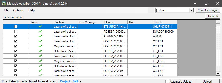
Figure 49. LIMS Uploader window
3. To manually upload files, check each file individually and clip upload. To automatically upload files, click on the Automatic Upload checkbox. The window can be minimized and MUT will be running in the background.
4. If files are marked by a purple question mark or red and white X icons, please contact a technician.
Purple question mark: Cannot identify the file.
Red and white X icons: Contains file errors.
5. Upon upload, data is moved to C:\DATA\Archive. If upload is unsuccessful, data is automatically moved to C:\DATA\Error. Please contact the PP technician is this occurs.
MUT Configuration
File Path
The file path MUT should look for files to upload is C: > data > IN. IMS writes upload files to C: > data > IN, so ensure the file path is set correctly. Note the uploaded files are written directly into the 'IN' folder. Images are not directly uploaded and are written to C: > data > IN > Images
Active Analyses
In MUT the 'active analyses' (Figure 50) should be set to Linescan Image, Processed RGB channels, and Whole-round Linescan. Linescan Image and Processed RGB Channels are for section half measurements. The Whole-Round Linescan Image is for 360 Imaging of hard rock cores. All three analyses should be set in the 'Active Uploaders' Column. Note it is ok for analyses to be in the 'Active Uploaders' even if MUT at that instrument host does not generate those files.
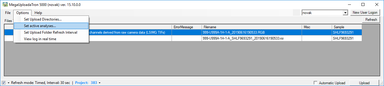
Figure 50. Select Set active analyses on MUT
Data File Formats
Two files are uploaded to LORE via MegaUploadaTron (MUT):
- .roi file : Contains callouts to the uncropped TIFF , uncropped JPEG, and cropped JPEG images. The images are linked files in LORE as Images > Core Closeup (LSIMG).
- .RGB file : Contains the red, green, and blue values calculated for each offset. The information is in LORE under Physical Properties > RGB Channels (RGB).
The files are independent of each other, both do not need to be present in order to upload, and often appear in MUT at different times.
MUT and .ini file
Be aware uploaded files have a callout for the .ini file. There is only one .ini file and the files will callout the .ini file currently present at the moment of uploading to LORE. If changes are made to settings that will alter the .ini and there are files piled up that have not uploaded to LORE, those files will upload the current .ini file, not the .ini file settings used for measurement. This implies files could have incorrect .ini files if rapid changes are made and users are not being careful.
Auxillary data Produced
The SHIL has the capability to produce two additional file types at the scientist's request:
- Hi RES RGB
- VCD-S
These files appear in separate folders in C: > data > in
Hi RES RGB: This file default is turned on and can be turned off in Instruments > Camera: General Setup (Figure 51). The Hi-Res RGB file reports a Red, Green, and Blue value for each line of pixels down the length of the core. 1cm is 200 lines of pixels so a 150cm core will yield approximately 30,000 lines of data depending on the exact crop length. The file is currently uploaded to the database (available in LORE under the expanded report Physical Properties > RGB Channels (RGB), rgb_high_res_asman_id column), and is instead copied to data1 at the end of the expedition.
VCD-S: The SHIL can preserve a digital copy of the VCD-S that is printed out. If a scientist wants to keep a digital copy of the scratch sheet turn on the feature in Instruments > Camera: VCDS Setup (Figure 51) . Files are then written to C: data > in > VCD-S. These files are not uploaded to LIMS and should be put in data1 at the end of the expedition. The files can be put on the server for scientist access to a convenient, shared location such as Uservol.
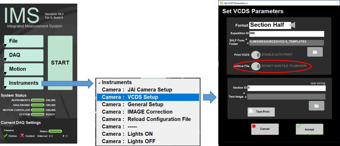
Figure 51. Select to preserve a digital copy of VCD-S
B. View and Verify Data
Data Available in LIVE
The data measured on each instrument can be viewed in real time on the LIMS information viewer (LIVE).
Choose the appropriate template (Ex: IMAGES_All), Expedition, Site, Hole or the needed restrictions and click View Data. The requested data will be displayed. You can travel in them by clicking on each of each core or section, which will enlarge the image.
Data Available in LORE
Each data set is written to a file by section. These reports are found under the Images heading and include: Core composites (COREPHOTO), core sections (LSIMG) and whole-round sections (WRLSC). The expanded reports include the linked original data files and more detailed information regarding the measurement.
Sample and Analysis Components
| Analysis | Component | Definition |
|---|---|---|
LSIMG (Core Section) | Exp | expedition number |
| Site | site number | |
| Hole | hole number | |
| Core | core number | |
| Type | type indicates the coring tool used to recover the core (typical types are F, H, R, X) | |
| Sect | section number | |
| A/W | archive (A) or working (W) section half | |
| Top Depth CSF-A (m) | location of the upper edge of the section expressed relative to the top of the hole. | |
| Bottom Depth CSF-A (m) | location of the lower edge of the section expressed relative to the top of the hole. | |
| Top Depth (other) (m) | location of the upper edge of the section expressed relative to the top of the hole. The location is presented in a scale selected by the science party or the report user. | |
| Bottom depth (other) (m) | location of the lower edge of the section expressed relative to the top of the hole. The location is presented in a scale selected by the science party or the report user. | |
| Display Status (T/F) | "T" (true) indicates that this image has been selected as the core section image to display in core descriptions and core composites. "F" (false) indicates that this image will not be displayed. (All images prior to Expedition 349 are designated as display images.) | |
| Uncropped image (JPG) link | link to URL of JPG version of core section image that shows the ruler and external space at the top and bottom of the section. | |
| Uncropped image filename | filename of uncropped image provided for identification purposes. | |
| Cropped image (JPG) link | link to URL of JPG version of core section image with the ruler and external space at the top and bottom of the section cropped. | |
| Cropped image filename | filename of cropped image provided for identification purposes. | |
| Timestamp (UTC) | point in time at which an observation or set of observations were made. Precise meaning of the value varies between systems due to variation in capability and/or implementation. | |
| Instrument | line-scan camera (e.g., JAICV107CL). | |
| Instrument group | Section Half Imaging Logger (SHIL). | |
| Text ID | automatically generated unique database identifier for a sample, visible on printed labels. | |
| Test No | Unique number associated with the instrument measurement steps that produced these data. | |
| Comments | observer's notes about the sample. |
| Analysis | Component | Definition |
|---|---|---|
| RGB Channels (RGB) | Exp | expedition number |
| Site | site number | |
| Hole | hole number | |
| Core | core number | |
| Type | type indicates the coring tool used to recover the core (typical types are F, H, R, X). | |
| Sect | section number | |
| A/W | archive (A) or working (W) section half. | |
| Offset (cm) | position of the observation made, measured relative to the top of a section. | |
| Depth CSF-A (m) | location of the observation expressed relative to the top of a hole. | |
| Depth (other) (m) | location of the observation expressed relative to the top of a hole. The location is presented in a scale selected by the science party or the report user. | |
| R | average of digitized red (R) channel over a user-defined rectangle along the core section. Values range from 0 to 255 (8-bit color digitization). | |
| G | average of digitized green (G) channel over a user-defined rectangle along the core section. Values range from 0 to 255 (8-bit color digitization). | |
| B | average of digitized blue (B) channel over a user-defined rectangle along the core section. Values range from 0 to 255 (8-bit color digitization). | |
| Timestamp (UTC) | point in time at which an observation or set of observations was made on the logger. | |
| Instrument | line-scan camera (e.g., JAICV107CL). | |
| Instrument Group | Section Half Imaging Logger (SHIL). | |
| Text ID | automatically generated unique database identifier for a sample, visible on printed labels. | |
| Test No | Unique number associated with the instrument measurement steps that produced these data. | |
| Comments | observer's notes about a measurement, the sample, or the measurement process. |
C. Retrieve Data from LIMS
Expedition data can be downloaded from the database using the instrument Expanded Report on Download LIMS core data (LORE).
IV. Important Notes
Glossary of Terms
Gain: a digital camera setting that controls the amplification of the signal from the camera sensor. It should be noted that this amplifies the whole signal, including any associated background noise.
Gamma: a digital camera setting that controls the grayscale reproduced on the image. An image gamma of unity indicates that the camera sensor is precisely reproducing the object gray scale (linear response). A gamma setting much greater than unity results in a silhouetted image in black and white.
White Balance: a camera setting that adjusts the color balance of light so that it appears a neutral white, and it is used to counteract the orange/yellow color of artificial light.
V. Appendix
A.1 Health, Safety & Environment
Safety
- These lights can get hot if the cooling fans are not used (cooling fans work automatically when lights come one). The temperature is shown on the LED read out above the camera and is set to maintain a temperature of 30 °C. During a section scan, the temperature will range between 30 and 35 °C. If Temperature goes above 50°C an alarm will sound. Caution is needed during the calibration process because the lights are stationary and remain on for much longer (during calibration the user controls Lights On/Lights Off). You can use the manual power switch to turn the lights on and off or the buttons in the software (the calibration procedure below uses the buttons in software). Use the heat resistant grey silicone mat for the shading and pixel corrections. Do not use the plastic Gray card. Make sure the temperature is maintained between 30 and 35°C for calibration (to match temperature of lights during imaging of a section).
- Never look at the LEDs directly. Even the reflected light can be painful. When working under the track make sure that the power is off.
- NOTE: if you are concerned with the heat dissipation on the core surface, you can use our FLIR cameras to confirm that the temperature is ok.
- Do not put your hands in or near the moving equipment. The actuators will torque out when impeded but injury could occur before that happens. Hardware abort buttons are located at both ends of the system for an emergency stop.
- Take care when working inside the electronics enclosure to avoid shocks from the power supply terminals.
Pollution Prevention
This procedure does not generate heat or gases and requires no containment equipment.
A.2 Maintenance and Troubleshooting
Troubleshooting
Common problems encountered when using the core imager and their possible causes and solutions:
Issue | Possible Causes | Solution |
Actuator squeal | NA | Lightly tap the actuator housing to silence the noise |
Image too dark | Manual F-stop on the camera closed down | Have technician adjust F-stop aperture |
Exposure time is too low | Increase exposure time | |
Focused lights are not aimed at the correct spot | Adjust lights | |
Track is “stuck” | Run was aborted with the software abort switch | Reset software and run sample again |
Run was aborted with the hardware abort switch | Reset hardware and run sample again | |
Gantry flag has tripped the end-of-travel limit switch | Adjust gantry flag and run sample again | |
Current limit on motors was exceeded | Check the Galil AMP-19520 for LED error indicators. Call track technician or ET to reset the motor controller | |
Torque limit on motors was exceeded. <we need to check how Labview handles this!>[djh1] | ||
Image indicates that camera was triggered erratically OR no image acquired | Camera was left in Free Run mode in MAX | Set camera to Externally Triggered for normal operation |
Linear encoder head has failed | Call an ET to verify/repair | |
Lens cap is on | Remove cap and repeat image capture procedure. | |
Exposure Intervals for Red, Green, and Blue are greater than the Line Trigger Interval | Adjust Exposure Intervals in JAI Camera Setup |
Maintenance
Frequency | Task |
|---|---|
Daily | Ensure that the color standards, ruler, and barcode imager lens are free from dust, smudges, and crumbs. |
Weekly | Using a mirror, ensure that there are no fingerprints or smudges on the camera lens. Call the imaging specialist if the lens needs cleaning. Do not attempt to clean it yourself! |
Monthly | Check socket head cap screws in the camera and lights mounting plates for looseness. |
Every Expedition |
|
Annually |
|
B.1 IMS Program Structure
a) IMS Program Structure
IMS is a modular program. Individual modules are as follows:
- Config Files: Unique for each track. Used for initialize the track and set up default parameters.
- Documents: Important Information related with configuration setup.
- Error: IMS error file.
- FRIENDS: Systems that use IMS but don't use DAQ Engine.
- IMS Common: Programs that are used by different instruments.
- PLUG-INS: Code for each of the instruments.
- Projects: Main IMS libraries.
- Resources: Other information and programs needed to run IMS.
- UI: User Interface
- X-CONFIG: .ini files, specifics for each instrument.
- MOTION plug-in: Codes for the motion control system.
- DAQ Engine: Code that organizes INST and MOTION plug-ins into a track system.
The IMS Main User Interface (IMS-UI) calls these modules, instructs them to initialize, and provides a user interface to their functionality.
b) Communication and Control Setup
Data communication and control is USB based and managed via National Instrument’s Measurement & Automation Explorer (NI-MAX). When you open NI-MAX and expand the Device and Interface section. The correct communications setup can be found at IMS Hardware Communications Setup.
B.2 Motion Control Setup
The track's push system consists of a NSK linear actuator driven by Schneider Electric stepping motor: MDrive23. The MDrive 23 is a high torque 1.8º integrated motor-driver-controller that connects to the PC via USB-RS485 cable. An IODP-built interface board (Figure 52) provides power control, emergency, limit/home switches, specialty I/O connections, and status lights. With the exception of a built in "Home" function, the MDive's IMS motion software module provides direct control of the motor's functions. The motor can be installed directly out of the box without any special preparation.
At IMS launch, a series of commands are sent to place the motor into a known state and then to search for the home switch and zero the encoder's position out put.
It is assumed that the hardware has been installed correctly and powered up. On the very first launch, a set of default values will be loaded that should get the track safely running. BUT BE READY to kill the motion using the Emergency-Stop button. Generally, a run-off is caused by incorrect scaling factors for the gear ratio, screw pitch, and or encoder counts per revolution. Setting these up correctly usually correct the issue.
Note: If the motor fails to initialize or locate the home switch, then an error will be reported. At this point, access the motion control utilities for trouble shooting. The START button will not appear and measurements are prevented.
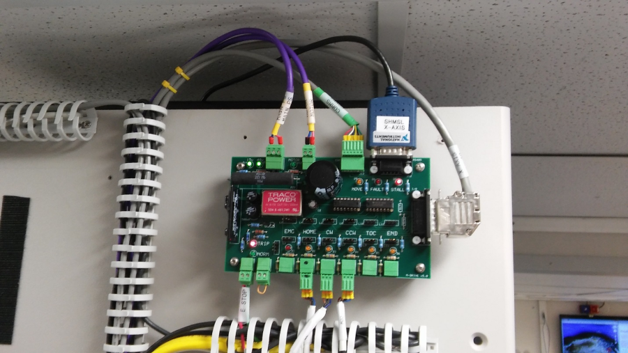
Figure 52. Interface board for motion control.
MDrive Setup
Select Setup from the Motion menu bar for MDrive Motion control window (Figure 53).
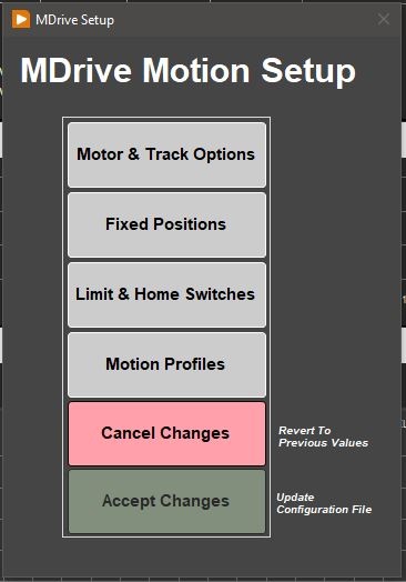
Figure 53. MDrive Motion Control window.
Track Options
Click Motor and Track Options to open the Track Motor Setup (Figure 54). Here is where the relationship between motor revolutions and linear motion of the track is defined.
Select Axis: In the case of the WRMSL and STMSL, it is always X.
Encoder Pulses/rev: Defined by the manufacturer of the MDrive as 2048.
Screw Pitch: Defined by the NSK actuator manufacturer as 2 cm/screw revolution.
Gear Ratio: In the current configuration, this is 4 to 1 but it can be changed.
Direction: The WRMSL is a right-hand track and a CCW rotation moves the pusher in a positive (from home to end of track) direction. The STMSL is a left-hand track so this value is set to CW. Now both are set as CCW.
Click Motion Utility to test these settings.
Click Accept to save the values or Cancel to return to the previous values.
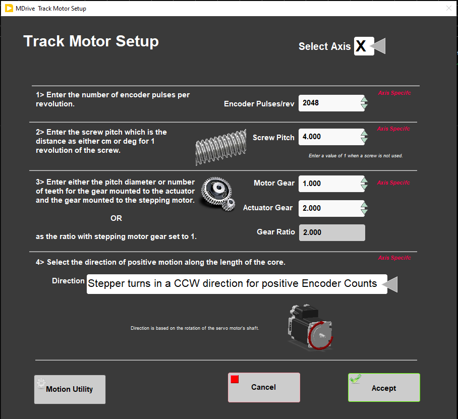
Figure 54. Track Motor Setup window.
Fixed Positions
Click Fixed Positions to open the Track Configuration window (Figure 56). In this window, define fixed track locations (Figure 57) used by IMS and enable the top of section (TOS) switch and the runout switch (ROS).
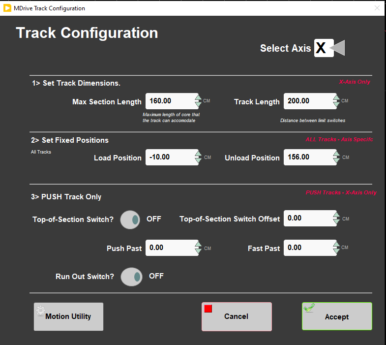
Figure 56. Track Configuration window.
Select Axis: In the case of the WRMSL and STMSL it is always X.
Max Section Length: Maximum length of section that can be placed in the track and still expect the track to handle and measure correctly. This value is set to 160 cm.
Track length: Distance in cm between the limit switches. Use the motion Utility to determine this value. This value is set to 200 cm.
Load and Unload: Offset in cm where the track will stop when ready to load a new section of core. In the case of both the WRMSL and STMSL, this the same as the home switch.
Top-of-Section Switch: THIS MUST ALWAYS BE enabled! The IMS software uses this switch to determine the physical length of the section, which is critical to the calculations that move the cores through the sensor. Without a TOS switch, the track is not functional.
Top-of-Section Switch Offset: Distance in cm from the home switch to the TOS switch. There is a utility under the DAQ > Find Top-of-Section Switch menu that will determine this value based on the current DAQ Move motion parameters (discussed in this section). ANY change in the motion profile requires that this utility be run because the final position (where the pusher bar stops) changes.
Push Past: The offset from the TOS where the pusher should stop. This value set the maximum measurement interval but MUST be several centimeters less than the distance from the TOS to the limit switch.
Fast Past: Distance the pusher will move at a higher speed before slowing down to find the TOS switch. This value MUST be several centimeters less than the distance from the TOS to the maximum section length with the pusher arm in the home position.
Run Out Switch: Switch at the end of the track that when enabled pauses the motion, preventing the section from being pushed onto the floor.
Click Motion Utility to test these settings. Click Accept to save the values or Cancel to return to the previous values.
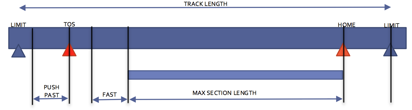
Figure 57. Schematic of fixed positions.
Limit and Home Switches
Click Limit and Home Switches to open Limit & Home Switches window (Figure 58).
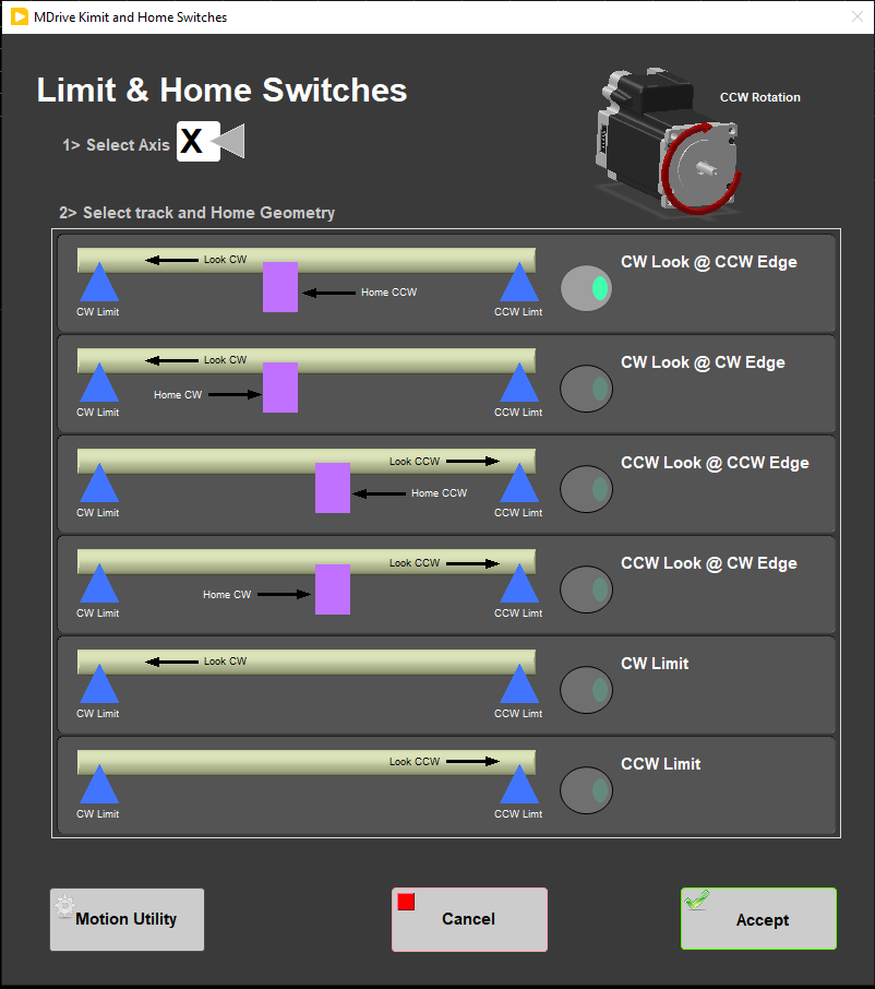
Figure 58. Limit & Home Switches window.
Select Axis: In the case of the WRMSL and STMSL it is always X.
The MDrive can be used with either a dedicated Home switch or a limit switch as a home switch. These tracks use the dedicated Home switch. Select the appropriate setup for the track in use. Use the Utilities to execute the Home command and verify the correct setting. If the home switch position of detection edge changes, verify the instrument offsets and relocate the TOS switch are still correct. Setting the edge from CW to CCW will change the offset by a least 1 cm.
Click Motion Utility to test these settings.
Click Accept to save the values or Cancel to return to the previous values.
Motion Profiles
Click Motion Profiles to open Motion Profiles window (Figure 59). The profiles are used to set the speed and acceleration profiles used by the track.
Setting the correct values for the motion profile takes a little experimentation to make the track run efficiently and safely.
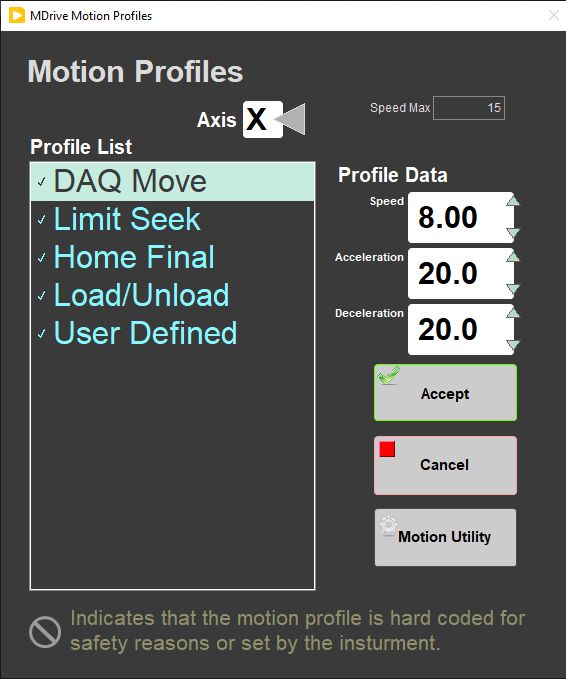
Figure 59. Motion Profile window.
DAQ Move: This profile controls moves between measurement positions. Set this to a reasonable speed with gradual acceleration so the pusher does not bump the sections.
Limit Seek: This profile finds the limit switch locations. Do not exceed 5 cm/sec and use a large deceleration value or the core could overrun the limit switch and hit the mechanical stop.
Home Final: This profile finds the final location of the home switch. Do not exceed 1 cm/sec and use a large deceleration value.
Load/Unload: This profile moves the pusher back to the load position. Set this to a reasonable but high speed with gradual acceleration and deceleration values. Setting this too slow will waste time, but keep safety in mind.
Push-Slow: This profile allows the pusher to move the new section into contact with the previous section and to locate the top of section. Use a speed a little less than the DAQ Move speed with slightly lower acceleration and deceleration values.
Push-Fast: This profile allows the pusher to move quickly to the TOS switch. Typically, it is set the same as the Load/Unload values.
User Define: This profile is used for testing only in the Motion Utilities program.
Click Motion Utility to test these settings.
Click Accept to save the values or Cancel to return to the previous values.
The following table shows the motion profile settings for the SHIL.
Axis→ | X-Axis | ||
|---|---|---|---|
Profile↓ | Speed | Accel. | Decel. |
DAQ Move | 8.0 | 20.0 | 20.0 |
Limit Seek | 3.0 | 5.0 | 30.0 |
Home Final | 0.5 | 2.0 | 30.0 |
Load/Unload | 30.0 | 5.0 | 5.0 |
User Defined | 20.0 | 10.0 | 30.0 |
Table: Motion Profile X-Axis for SHIL
B.3 LIMS Component Tables
The following LIMS component tables are included under the Section Half Imaging Logger (SHIL):
- LSIMG - linescan imaging of the section half
- RGB - red/green/blue analysis of the LSIMG TIF, usually in 2 cm wide (Y-axis) x 0.5 cm deep (Z-axis) bins at the Y-axis center of the section
- WRLS - linescan imaging of the individual 90-degree quadrants for whole-round imaging of the outside of a hard rock section
- WRLSC - component for the collection of the final 90-degree quadrant images as well as the 360-degree composite image
| ANALYSIS | TABLE | NAME | ABOUT TEXT |
| LSIMG | SAMPLE | Exp | Exp: expedition number |
| LSIMG | SAMPLE | Site | Site: site number |
| LSIMG | SAMPLE | Hole | Hole: hole number |
| LSIMG | SAMPLE | Core | Core: core number |
| LSIMG | SAMPLE | Type | Type: type indicates the coring tool used to recover the core (typical types are F, H, R, X). |
| LSIMG | SAMPLE | Sect | Sect: section number |
| LSIMG | SAMPLE | A/W | A/W: archive (A) or working (W) section half. |
| LSIMG | SAMPLE | text_id | Text_ID: automatically generated database identifier for a sample, also carried on the printed labels. This identifier is guaranteed to be unique across all samples. |
| LSIMG | SAMPLE | sample_number | Sample Number: automatically generated database identifier for a sample. This is the primary key of the SAMPLE table. |
| LSIMG | SAMPLE | label_id | Label identifier: automatically generated, human readable name for a sample that is printed on labels. This name is not guaranteed unique across all samples. |
| LSIMG | SAMPLE | sample_name | Sample name: short name that may be specified for a sample. You can use an advanced filter to narrow your search by this parameter. |
| LSIMG | SAMPLE | x_sample_state | Sample state: Single-character identifier always set to "W" for samples; standards can vary. |
| LSIMG | SAMPLE | x_project | Project: similar in scope to the expedition number, the difference being that the project is the current cruise, whereas expedition could refer to material/results obtained on previous cruises |
| LSIMG | SAMPLE | x_capt_loc | Captured location: "captured location," this field is usually null and is unnecessary because any sample captured on the JR has a sample_number ending in 1, and GCR ending in 2 |
| LSIMG | SAMPLE | location | Location: location that sample was taken; this field is usually null and is unnecessary because any sample captured on the JR has a sample_number ending in 1, and GCR ending in 2 |
| LSIMG | SAMPLE | x_sampling_tool | Sampling tool: sampling tool used to take the sample (e.g., syringe, spatula) |
| LSIMG | SAMPLE | changed_by | Changed by: username of account used to make a change to a sample record |
| LSIMG | SAMPLE | changed_on | Changed on: date/time stamp for change made to a sample record |
| LSIMG | SAMPLE | sample_type | Sample type: type of sample from a predefined list (e.g., HOLE, CORE, LIQ) |
| LSIMG | SAMPLE | x_offset | Offset (m): top offset of sample from top of parent sample, expressed in meters. |
| LSIMG | SAMPLE | x_offset_cm | Offset (cm): top offset of sample from top of parent sample, expressed in centimeters. This is a calculated field (offset, converted to cm) |
| LSIMG | SAMPLE | x_bottom_offset_cm | Bottom offset (cm): bottom offset of sample from top of parent sample, expressed in centimeters. This is a calculated field (offset + length, converted to cm) |
| LSIMG | SAMPLE | x_diameter | Diameter (cm): diameter of sample, usually applied only to CORE, SECT, SHLF, and WRND samples; however this field is null on both Exp. 390 and 393, so it is no longer populated by Sample Master |
| LSIMG | SAMPLE | x_orig_len | Original length (m): field for the original length of a sample; not always (or reliably) populated |
| LSIMG | SAMPLE | x_length | Length (m): field for the length of a sample [as entered upon creation] |
| LSIMG | SAMPLE | x_length_cm | Length (cm): field for the length of a sample. This is a calculated field (length, converted to cm). |
| LSIMG | SAMPLE | status | Status: single-character code for the current status of a sample (e.g., active, canceled) |
| LSIMG | SAMPLE | old_status | Old status: single-character code for the previous status of a sample; used by the LIME program to restore a canceled sample |
| LSIMG | SAMPLE | original_sample | Original sample: field tying a sample below the CORE level to its parent HOLE sample |
| LSIMG | SAMPLE | parent_sample | Parent sample: the sample from which this sample was taken (e.g., for PWDR samples, this might be a SHLF or possibly another PWDR) |
| LSIMG | SAMPLE | standard | Standard: T/F field to differentiate between samples (standard=F) and QAQC standards (standard=T) |
| LSIMG | SAMPLE | login_by | Login by: username of account used to create the sample (can be the LIMS itself [e.g., SHLFs created when a SECT is created]) |
| LSIMG | SAMPLE | login_date | Login date: creation date of the sample |
| LSIMG | SAMPLE | legacy | Legacy flag: T/F indicator for when a sample is from a previous expedition and is locked/uneditable on this expedition |
| LSIMG | TEST | test changed_on | TEST changed on: date/time stamp for a change to a test record. |
| LSIMG | TEST | test status | TEST status: single-character code for the current status of a test (e.g., active, in process, canceled) |
| LSIMG | TEST | test old_status | TEST old status: single-character code for the previous status of a test; used by the LIME program to restore a canceled test |
| LSIMG | TEST | test test_number | TEST test number: automatically generated database identifier for a test record. This is the primary key of the TEST table. |
| LSIMG | TEST | test date_received | TEST date received: date/time stamp for the creation of the test record. |
| LSIMG | TEST | test instrument | TEST instrument [instrument group]: field that describes the instrument group (most often this applies to loggers with multiple sensors); often obscure (e.g., user_input) |
| LSIMG | TEST | test analysis | TEST analysis: analysis code associated with this test (foreign key to the ANALYSIS table) |
| LSIMG | TEST | test x_project | TEST project: similar in scope to the expedition number, the difference being that the project is the current cruise, whereas expedition could refer to material/results obtained on previous cruises |
| LSIMG | TEST | test sample_number | TEST sample number: the sample_number of the sample to which this test record is attached; a foreign key to the SAMPLE table |
| LSIMG | TEST | test x_display | TEST display flag: T/F field to indicate whether an image is the display image |
| LSIMG | TEST | test legacy | TEST legacy: T/F indicator for when a test from a previous expedition and is locked/uneditable on this expedition |
| LSIMG | CALCULATED | Top depth CSF-A (m) | Top depth CSF-A (m): position of observation expressed relative to the top of the hole. |
| LSIMG | CALCULATED | Bottom depth CSF-A (m) | Bottom depth CSF-A (m): position of observation expressed relative to the top of the hole. |
| LSIMG | CALCULATED | Top depth CSF-B (m) | Top depth [other] (m): position of observation expressed relative to the top of the hole. The location is presented in a scale selected by the science party or the report user. |
| LSIMG | CALCULATED | Bottom depth CSF-B (m) | Bottom depth [other] (m): position of observation expressed relative to the top of the hole. The location is presented in a scale selected by the science party or the report user. |
| LSIMG | RESULT | config_asman_id | RESULT configuration file ASMAN_ID: serial number of the ASMAN link for the configuration file |
| LSIMG | RESULT | config_filename | RESULT configuration filename: file name of the configuration file |
| LSIMG | RESULT | consumer_image_asman_id | RESULT consumer image ASMAN_ID: serial number of the ASMAN link for the uncropped JPG image file |
| LSIMG | RESULT | consumer_image_filename | RESULT consumer image filename: file name of the uncropped JPG image file |
| LSIMG | RESULT | correction | RESULT correction: summary of corrections applied to the TIF file and JPG file (contrast, gamma, and brightness only) |
| LSIMG | RESULT | cropped_image_asman_id | RESULT cropped image ASMAN_ID: serial number of the ASMAN link for the cropped JPG image file |
| LSIMG | RESULT | cropped_image_filename | RESULT cropped image filename: file name of the cropped JPG image file |
| LSIMG | RESULT | cropped_image_length | RESULT cropped image length (cm): length of the cropped image as calculated from the total lines x 50 micron pixels |
| LSIMG | RESULT | image_description | RESULT image description: archaic field for "Pristine" or other choices |
| LSIMG | RESULT | image_purpose | RESULT image purpose: field for what the target is (e.g., soft sediment, dry hard rock) |
| LSIMG | RESULT | instrument | RESULT instrument: which sensor is used for this result; for LSIMG it is currently JAI SW-2001T-CL-F camera |
| LSIMG | RESULT | observed_length | RESULT observed length (cm): length of the core section as entered by the operator |
| LSIMG | RESULT | original_image_asman_id | RESULT original image ASMAN_ID: serial number of the ASMAn link for the uncropped TIF file (also not adjusted for contrast, gamma, or brightness) |
| LSIMG | RESULT | original_image_filename | RESULT original image filename: file name of the uncropped TIF file |
| LSIMG | RESULT | roi_left_edge | RESULT region of interest left edge (pixels): position of the left edge of the cropped image in pixels |
| LSIMG | RESULT | roi_lower_edge | RESULT region of interest lower edge (pixels): position of the lower edge of the cropped image in pixels |
| LSIMG | RESULT | roi_right_edge | RESULT region of interest right edge (pixels): position of the right edge of the cropped image in pixels |
| LSIMG | RESULT | roi_upper_edge | RESULT region of interest upper edge (pixels): position of the upper edge of the cropped image in pixels |
| LSIMG | RESULT | run_asman_id | RESULT run file ASMAN_ID: serial number of the ASMAN link for the run (.ROI) file |
| LSIMG | RESULT | run_filename | RESULT run filename: file name for the run (.ROI) file |
| LSIMG | SAMPLE | sample description | SAMPLE comment: contents of the SAMPLE.description field, usually shown on reports as "Sample comments" |
| LSIMG | TEST | test test_comment | TEST comment: contents of the TEST.comment field, usually shown on reports as "Test comments" |
| LSIMG | RESULT | result comments | RESULT comment: contents of a result parameter with name = "comment," usually shown on reports as "Result comments" |
| ANALYSIS | TABLE | NAME | ABOUT TEXT |
| RGB | SAMPLE | Exp | Exp: expedition number |
| RGB | SAMPLE | Site | Site: site number |
| RGB | SAMPLE | Hole | Hole: hole number |
| RGB | SAMPLE | Core | Core: core number |
| RGB | SAMPLE | Type | Type: type indicates the coring tool used to recover the core (typical types are F, H, R, X). |
| RGB | SAMPLE | Sect | Sect: section number |
| RGB | SAMPLE | A/W | A/W: archive (A) or working (W) section half. |
| RGB | SAMPLE | text_id | Text_ID: automatically generated database identifier for a sample, also carried on the printed labels. This identifier is guaranteed to be unique across all samples. |
| RGB | SAMPLE | sample_number | Sample Number: automatically generated database identifier for a sample. This is the primary key of the SAMPLE table. |
| RGB | SAMPLE | label_id | Label identifier: automatically generated, human readable name for a sample that is printed on labels. This name is not guaranteed unique across all samples. |
| RGB | SAMPLE | sample_name | Sample name: short name that may be specified for a sample. You can use an advanced filter to narrow your search by this parameter. |
| RGB | SAMPLE | x_sample_state | Sample state: Single-character identifier always set to "W" for samples; standards can vary. |
| RGB | SAMPLE | x_project | Project: similar in scope to the expedition number, the difference being that the project is the current cruise, whereas expedition could refer to material/results obtained on previous cruises |
| RGB | SAMPLE | x_capt_loc | Captured location: "captured location," this field is usually null and is unnecessary because any sample captured on the JR has a sample_number ending in 1, and GCR ending in 2 |
| RGB | SAMPLE | location | Location: location that sample was taken; this field is usually null and is unnecessary because any sample captured on the JR has a sample_number ending in 1, and GCR ending in 2 |
| RGB | SAMPLE | x_sampling_tool | Sampling tool: sampling tool used to take the sample (e.g., syringe, spatula) |
| RGB | SAMPLE | changed_by | Changed by: username of account used to make a change to a sample record |
| RGB | SAMPLE | changed_on | Changed on: date/time stamp for change made to a sample record |
| RGB | SAMPLE | sample_type | Sample type: type of sample from a predefined list (e.g., HOLE, CORE, LIQ) |
| RGB | SAMPLE | x_offset | Offset (m): top offset of sample from top of parent sample, expressed in meters. |
| RGB | SAMPLE | x_offset_cm | Offset (cm): top offset of sample from top of parent sample, expressed in centimeters. This is a calculated field (offset, converted to cm) |
| RGB | SAMPLE | x_bottom_offset_cm | Bottom offset (cm): bottom offset of sample from top of parent sample, expressed in centimeters. This is a calculated field (offset + length, converted to cm) |
| RGB | SAMPLE | x_diameter | Diameter (cm): diameter of sample, usually applied only to CORE, SECT, SHLF, and WRND samples; however this field is null on both Exp. 390 and 393, so it is no longer populated by Sample Master |
| RGB | SAMPLE | x_orig_len | Original length (m): field for the original length of a sample; not always (or reliably) populated |
| RGB | SAMPLE | x_length | Length (m): field for the length of a sample [as entered upon creation] |
| RGB | SAMPLE | x_length_cm | Length (cm): field for the length of a sample. This is a calculated field (length, converted to cm). |
| RGB | SAMPLE | status | Status: single-character code for the current status of a sample (e.g., active, canceled) |
| RGB | SAMPLE | old_status | Old status: single-character code for the previous status of a sample; used by the LIME program to restore a canceled sample |
| RGB | SAMPLE | original_sample | Original sample: field tying a sample below the CORE level to its parent HOLE sample |
| RGB | SAMPLE | parent_sample | Parent sample: the sample from which this sample was taken (e.g., for PWDR samples, this might be a SHLF or possibly another PWDR) |
| RGB | SAMPLE | standard | Standard: T/F field to differentiate between samples (standard=F) and QAQC standards (standard=T) |
| RGB | SAMPLE | login_by | Login by: username of account used to create the sample (can be the LIMS itself [e.g., SHLFs created when a SECT is created]) |
| RGB | SAMPLE | login_date | Login date: creation date of the sample |
| RGB | SAMPLE | legacy | Legacy flag: T/F indicator for when a sample is from a previous expedition and is locked/uneditable on this expedition |
| RGB | TEST | test changed_on | TEST changed on: date/time stamp for a change to a test record. |
| RGB | TEST | test status | TEST status: single-character code for the current status of a test (e.g., active, in process, canceled) |
| RGB | TEST | test old_status | TEST old status: single-character code for the previous status of a test; used by the LIME program to restore a canceled test |
| RGB | TEST | test test_number | TEST test number: automatically generated database identifier for a test record. This is the primary key of the TEST table. |
| RGB | TEST | test date_received | TEST date received: date/time stamp for the creation of the test record. |
| RGB | TEST | test instrument | TEST instrument [instrument group]: field that describes the instrument group (most often this applies to loggers with multiple sensors); often obscure (e.g., user_input) |
| RGB | TEST | test analysis | TEST analysis: analysis code associated with this test (foreign key to the ANALYSIS table) |
| RGB | TEST | test x_project | TEST project: similar in scope to the expedition number, the difference being that the project is the current cruise, whereas expedition could refer to material/results obtained on previous cruises |
| RGB | TEST | test sample_number | TEST sample number: the sample_number of the sample to which this test record is attached; a foreign key to the SAMPLE table |
| RGB | CALCULATED | Depth CSF-A (m) | Depth CSF-A (m): position of observation expressed relative to the top of the hole. |
| RGB | CALCULATED | Depth CSF-B (m) | Depth [other] (m): position of observation expressed relative to the top of the hole. The location is presented in a scale selected by the science party or the report user. |
| RGB | RESULT | red | RESULT red (R) channel: average of digitized red (R) channel over a user-defined rectangle along the core section. Values range from 0 to 255 (8-bit color digitization). |
| RGB | RESULT | green | RESULT green (G) channel: average of digitized green (G) channel over a user-defined rectangle along the core section. Values range from 0 to 255 (8-bit color digitization). |
| RGB | RESULT | blue | RESULT blue (B) channel: average of digitized blue (B) channel over a user-defined rectangle along the core section. Values range from 0 to 255 (8-bit color digitization). |
| RGB | RESULT | config_asman_id | RESULT config file ASMAN_ID: serial number of the ASMAN link for the configuration file |
| RGB | RESULT | config_filename | RESULT config filename: file name of the configuration file |
| RGB | RESULT | observed_length (cm) | RESULT observed length (cm): length of the section as recorded by the core logger track |
| RGB | RESULT | offset (cm) | RESULT offset (cm): position of the observation made, measured relative to the top of a section half. |
| RGB | RESULT | run_asman_id | RESULT run file ASMAN_ID: serial number of the ASMAN link for the run (.RGB) file |
| RGB | RESULT | run_filename | RESULT run filename: file name of the run (.RGB) file |
| RGB | RESULT | rgb_high_res_asman_id | RESULT high res RGB ASMAN_ID: serial number of the ASMAN link for the high resolution RGB (.DAT) file |
| RGB | RESULT | rgb_high_res_filename | RESULT high res RGB filename: filename for the high resolution RGB (.DAT) file |
| RGB | SAMPLE | sample description | SAMPLE comment: contents of the SAMPLE.description field, usually shown on reports as "Sample comments" |
| RGB | TEST | test test_comment | TEST comment: contents of the TEST.comment field, usually shown on reports as "Test comments" |
| RGB | RESULT | result comments | RESULT comment: contents of a result parameter with name = "comment," usually shown on reports as "Result comments" |
| ANALYSIS | TABLE | NAME | ABOUT TEXT |
| WRLS | SAMPLE | Exp | Exp: expedition number |
| WRLS | SAMPLE | Site | Site: site number |
| WRLS | SAMPLE | Hole | Hole: hole number |
| WRLS | SAMPLE | Core | Core: core number |
| WRLS | SAMPLE | Type | Type: type indicates the coring tool used to recover the core (typical types are F, H, R, X). |
| WRLS | SAMPLE | Sect | Sect: section number |
| WRLS | SAMPLE | text_id | Text_ID: automatically generated database identifier for a sample, also carried on the printed labels. This identifier is guaranteed to be unique across all samples. |
| WRLS | SAMPLE | sample_number | Sample Number: automatically generated database identifier for a sample. This is the primary key of the SAMPLE table. |
| WRLS | SAMPLE | label_id | Label identifier: automatically generated, human readable name for a sample that is printed on labels. This name is not guaranteed unique across all samples. |
| WRLS | SAMPLE | sample_name | Sample name: short name that may be specified for a sample. You can use an advanced filter to narrow your search by this parameter. |
| WRLS | SAMPLE | x_sample_state | Sample state: Single-character identifier always set to "W" for samples; standards can vary. |
| WRLS | SAMPLE | x_project | Project: similar in scope to the expedition number, the difference being that the project is the current cruise, whereas expedition could refer to material/results obtained on previous cruises |
| WRLS | SAMPLE | x_capt_loc | Captured location: "captured location," this field is usually null and is unnecessary because any sample captured on the JR has a sample_number ending in 1, and GCR ending in 2 |
| WRLS | SAMPLE | location | Location: location that sample was taken; this field is usually null and is unnecessary because any sample captured on the JR has a sample_number ending in 1, and GCR ending in 2 |
| WRLS | SAMPLE | x_sampling_tool | Sampling tool: sampling tool used to take the sample (e.g., syringe, spatula) |
| WRLS | SAMPLE | changed_by | Changed by: username of account used to make a change to a sample record |
| WRLS | SAMPLE | changed_on | Changed on: date/time stamp for change made to a sample record |
| WRLS | SAMPLE | sample_type | Sample type: type of sample from a predefined list (e.g., HOLE, CORE, LIQ) |
| WRLS | SAMPLE | x_offset | Offset (m): top offset of sample from top of parent sample, expressed in meters. |
| WRLS | SAMPLE | x_offset_cm | Offset (cm): top offset of sample from top of parent sample, expressed in centimeters. This is a calculated field (offset, converted to cm) |
| WRLS | SAMPLE | x_bottom_offset_cm | Bottom offset (cm): bottom offset of sample from top of parent sample, expressed in centimeters. This is a calculated field (offset + length, converted to cm) |
| WRLS | SAMPLE | x_diameter | Diameter (cm): diameter of sample, usually applied only to CORE, SECT, SHLF, and WRND samples; however this field is null on both Exp. 390 and 393, so it is no longer populated by Sample Master |
| WRLS | SAMPLE | x_orig_len | Original length (m): field for the original length of a sample; not always (or reliably) populated |
| WRLS | SAMPLE | x_length | Length (m): field for the length of a sample [as entered upon creation] |
| WRLS | SAMPLE | x_length_cm | Length (cm): field for the length of a sample. This is a calculated field (length, converted to cm). |
| WRLS | SAMPLE | status | Status: single-character code for the current status of a sample (e.g., active, canceled) |
| WRLS | SAMPLE | old_status | Old status: single-character code for the previous status of a sample; used by the LIME program to restore a canceled sample |
| WRLS | SAMPLE | original_sample | Original sample: field tying a sample below the CORE level to its parent HOLE sample |
| WRLS | SAMPLE | parent_sample | Parent sample: the sample from which this sample was taken (e.g., for PWDR samples, this might be a SHLF or possibly another PWDR) |
| WRLS | SAMPLE | standard | Standard: T/F field to differentiate between samples (standard=F) and QAQC standards (standard=T) |
| WRLS | SAMPLE | login_by | Login by: username of account used to create the sample (can be the LIMS itself [e.g., SHLFs created when a SECT is created]) |
| WRLS | SAMPLE | login_date | Login date: creation date of the sample |
| WRLS | SAMPLE | legacy | Legacy flag: T/F indicator for when a sample is from a previous expedition and is locked/uneditable on this expedition |
| WRLS | TEST | test changed_on | TEST changed on: date/time stamp for a change to a test record. |
| WRLS | TEST | test status | TEST status: single-character code for the current status of a test (e.g., active, in process, canceled) |
| WRLS | TEST | test old_status | TEST old status: single-character code for the previous status of a test; used by the LIME program to restore a canceled test |
| WRLS | TEST | test test_number | TEST test number: automatically generated database identifier for a test record. This is the primary key of the TEST table. |
| WRLS | TEST | test date_received | TEST date received: date/time stamp for the creation of the test record. |
| WRLS | TEST | test instrument | TEST instrument [instrument group]: field that describes the instrument group (most often this applies to loggers with multiple sensors); often obscure (e.g., user_input) |
| WRLS | TEST | test analysis | TEST analysis: analysis code associated with this test (foreign key to the ANALYSIS table) |
| WRLS | TEST | test x_project | TEST project: similar in scope to the expedition number, the difference being that the project is the current cruise, whereas expedition could refer to material/results obtained on previous cruises |
| WRLS | TEST | test sample_number | TEST sample number: the sample_number of the sample to which this test record is attached; a foreign key to the SAMPLE table |
| WRLS | TEST | test x_display | TEST display flag: T/F field to indicate whether an image is the display image |
| WRLS | TEST | test legacy | TEST legacy: T/F indicator for when a test from a previous expedition and is locked/uneditable on this expedition |
| WRLS | CALCULATED | Top depth CSF-A (m) | Top depth CSF-A (m): position of observation expressed relative to the top of the hole. |
| WRLS | CALCULATED | Bottom depth CSF-A (m) | Bottom depth CSF-A (m): position of observation expressed relative to the top of the hole. |
| WRLS | CALCULATED | Top depth CSF-B (m) | Top depth [other] (m): position of observation expressed relative to the top of the hole. The location is presented in a scale selected by the science party or the report user. |
| WRLS | CALCULATED | Bottom depth CSF-B (m) | Bottom depth [other] (m): position of observation expressed relative to the top of the hole. The location is presented in a scale selected by the science party or the report user. |
| WRLS | RESULT | quadrant | RESULT quadrant: which 90-degree quadrant was captured in this image |
| WRLS | RESULT | quadrant_tif_asman_id | RESULT quadrant TIF ASMAN_ID: serial number of the ASMAN link for the quadrant TIF/TIFF image |
| WRLS | RESULT | quadrant_tif_filename | RESULT quadrant TIF filename: file name of the quadrant TIF/TIFF image |
| WRLS | RESULT | quadrant_jpg_asman_id | RESULT quadrant JPG ASMAN_ID: serial number of the ASMAN link for the quadrant JPG/JPEG image |
| WRLS | RESULT | quadrant_jpg_filename | RESULT quadrant JPG filename: file name of the quadrant JPG/JPEG image |
| WRLS | RESULT | run_asman_id | RESULT run file ASMAN_ID: serial number of the ASMAN link for the run (.WRLS) file |
| WRLS | RESULT | run_filename | RESULT run filename: file name of the run (.WRLS) file |
| WRLS | SAMPLE | sample description | SAMPLE comment: contents of the SAMPLE.description field, usually shown on reports as "Sample comments" |
| WRLS | TEST | test test_comment | TEST comment: contents of the TEST.comment field, usually shown on reports as "Test comments" |
| WRLS | RESULT | result comments | RESULT comment: contents of a result parameter with name = "comment," usually shown on reports as "Result comments" |
| ANALYSIS | TABLE | NAME | ABOUT TEXT |
| WRLSC | SAMPLE | Exp | Exp: expedition number |
| WRLSC | SAMPLE | Site | Site: site number |
| WRLSC | SAMPLE | Hole | Hole: hole number |
| WRLSC | SAMPLE | Core | Core: core number |
| WRLSC | SAMPLE | Type | Type: type indicates the coring tool used to recover the core (typical types are F, H, R, X). |
| WRLSC | SAMPLE | Sect | Sect: section number |
| WRLSC | SAMPLE | text_id | Text_ID: automatically generated database identifier for a sample, also carried on the printed labels. This identifier is guaranteed to be unique across all samples. |
| WRLSC | SAMPLE | sample_number | Sample Number: automatically generated database identifier for a sample. This is the primary key of the SAMPLE table. |
| WRLSC | SAMPLE | label_id | Label identifier: automatically generated, human readable name for a sample that is printed on labels. This name is not guaranteed unique across all samples. |
| WRLSC | SAMPLE | sample_name | Sample name: short name that may be specified for a sample. You can use an advanced filter to narrow your search by this parameter. |
| WRLSC | SAMPLE | x_sample_state | Sample state: Single-character identifier always set to "W" for samples; standards can vary. |
| WRLSC | SAMPLE | x_project | Project: similar in scope to the expedition number, the difference being that the project is the current cruise, whereas expedition could refer to material/results obtained on previous cruises |
| WRLSC | SAMPLE | x_capt_loc | Captured location: "captured location," this field is usually null and is unnecessary because any sample captured on the JR has a sample_number ending in 1, and GCR ending in 2 |
| WRLSC | SAMPLE | location | Location: location that sample was taken; this field is usually null and is unnecessary because any sample captured on the JR has a sample_number ending in 1, and GCR ending in 2 |
| WRLSC | SAMPLE | x_sampling_tool | Sampling tool: sampling tool used to take the sample (e.g., syringe, spatula) |
| WRLSC | SAMPLE | changed_by | Changed by: username of account used to make a change to a sample record |
| WRLSC | SAMPLE | changed_on | Changed on: date/time stamp for change made to a sample record |
| WRLSC | SAMPLE | sample_type | Sample type: type of sample from a predefined list (e.g., HOLE, CORE, LIQ) |
| WRLSC | SAMPLE | x_offset | Offset (m): top offset of sample from top of parent sample, expressed in meters. |
| WRLSC | SAMPLE | x_offset_cm | Offset (cm): top offset of sample from top of parent sample, expressed in centimeters. This is a calculated field (offset, converted to cm) |
| WRLSC | SAMPLE | x_bottom_offset_cm | Bottom offset (cm): bottom offset of sample from top of parent sample, expressed in centimeters. This is a calculated field (offset + length, converted to cm) |
| WRLSC | SAMPLE | x_diameter | Diameter (cm): diameter of sample, usually applied only to CORE, SECT, SHLF, and WRND samples; however this field is null on both Exp. 390 and 393, so it is no longer populated by Sample Master |
| WRLSC | SAMPLE | x_orig_len | Original length (m): field for the original length of a sample; not always (or reliably) populated |
| WRLSC | SAMPLE | x_length | Length (m): field for the length of a sample [as entered upon creation] |
| WRLSC | SAMPLE | x_length_cm | Length (cm): field for the length of a sample. This is a calculated field (length, converted to cm). |
| WRLSC | SAMPLE | status | Status: single-character code for the current status of a sample (e.g., active, canceled) |
| WRLSC | SAMPLE | old_status | Old status: single-character code for the previous status of a sample; used by the LIME program to restore a canceled sample |
| WRLSC | SAMPLE | original_sample | Original sample: field tying a sample below the CORE level to its parent HOLE sample |
| WRLSC | SAMPLE | parent_sample | Parent sample: the sample from which this sample was taken (e.g., for PWDR samples, this might be a SHLF or possibly another PWDR) |
| WRLSC | SAMPLE | standard | Standard: T/F field to differentiate between samples (standard=F) and QAQC standards (standard=T) |
| WRLSC | SAMPLE | login_by | Login by: username of account used to create the sample (can be the LIMS itself [e.g., SHLFs created when a SECT is created]) |
| WRLSC | SAMPLE | login_date | Login date: creation date of the sample |
| WRLSC | SAMPLE | legacy | Legacy flag: T/F indicator for when a sample is from a previous expedition and is locked/uneditable on this expedition |
| WRLSC | TEST | test changed_on | TEST changed on: date/time stamp for a change to a test record. |
| WRLSC | TEST | test status | TEST status: single-character code for the current status of a test (e.g., active, in process, canceled) |
| WRLSC | TEST | test old_status | TEST old status: single-character code for the previous status of a test; used by the LIME program to restore a canceled test |
| WRLSC | TEST | test test_number | TEST test number: automatically generated database identifier for a test record. This is the primary key of the TEST table. |
| WRLSC | TEST | test date_received | TEST date received: date/time stamp for the creation of the test record. |
| WRLSC | TEST | test instrument | TEST instrument [instrument group]: field that describes the instrument group (most often this applies to loggers with multiple sensors); often obscure (e.g., user_input) |
| WRLSC | TEST | test analysis | TEST analysis: analysis code associated with this test (foreign key to the ANALYSIS table) |
| WRLSC | TEST | test x_project | TEST project: similar in scope to the expedition number, the difference being that the project is the current cruise, whereas expedition could refer to material/results obtained on previous cruises |
| WRLSC | TEST | test sample_number | TEST sample number: the sample_number of the sample to which this test record is attached; a foreign key to the SAMPLE table |
| WRLSC | TEST | test x_display | TEST display flag: T/F field to indicate whether an image is the display image |
| WRLSC | TEST | test legacy | TEST legacy: T/F indicator for when a test from a previous expedition and is locked/uneditable on this expedition |
| WRLSC | CALCULATED | Top depth CSF-A (m) | Top depth CSF-A (m): position of observation expressed relative to the top of the hole. |
| WRLSC | CALCULATED | Bottom depth CSF-A (m) | Bottom depth CSF-A (m): position of observation expressed relative to the top of the hole. |
| WRLSC | CALCULATED | Top depth CSF-B (m) | Top depth [other] (m): position of observation expressed relative to the top of the hole. The location is presented in a scale selected by the science party or the report user. |
| WRLSC | CALCULATED | Bottom depth CSF-B (m) | Bottom depth [other] (m): position of observation expressed relative to the top of the hole. The location is presented in a scale selected by the science party or the report user. |
| WRLSC | RESULT | jpg0_asman_id | RESULT 0 degree JPG ASMAN_ID: serial number of the ASMAN link for the 0-degree quadrant JPG/JPEG image |
| WRLSC | RESULT | jpg90_asman_id | RESULT 90 degree JPG ASMAN_ID: serial number of the ASMAN link for the 90-degree quadrant JPG/JPEG image |
| WRLSC | RESULT | jpg180_asman_id | RESULT 180 degree JPG ASMAN_ID: serial number of the ASMAN link for the 180-degree quadrant JPG/JPEG image |
| WRLSC | RESULT | jpg270_asman_id | RESULT 270 degree JPG ASMAN_ID: serial number of the ASMAN link for the 270-degree quadrant JPG/JPEG image |
| WRLSC | RESULT | jpg360_asman_id | RESULT 360 degree image JPG ASMAN_ID: serial number of the composite 360-degree image JPG/JPEG image |
| WRLSC | RESULT | jpg360_filename | RESULT 360 degree JPG filename: file name of the composite 360-degree JPG/JPEG image (a filename exists for each quadrant, but name is similar enough it was omitted from expanded report) |
| WRLSC | RESULT | tif0_asman_id | RESULT 0 degree TIF ASMAN_ID: serial number of the ASMAN link for the 0-degree quadrant TIF/TIFF image |
| WRLSC | RESULT | tif90_asman_id | RESULT 90 degree TIF ASMAN_ID: serial number of the ASMAN link for the 90-degree quadrant TIF/TIFF image |
| WRLSC | RESULT | tif180_asman_id | RESULT 180 degree TIF ASMAN_ID: serial number of the ASMAN link for the 180-degree quadrant TIF/TIFF image |
| WRLSC | RESULT | tif270_asman_id | RESULT 270 degree TIF ASMAN_ID: serial number of the ASMAN link for the 270-degree quadrant TIF/TIFF image |
| WRLSC | RESULT | tif360_asman_id | RESULT 360 degree image TIF ASMAN_ID: serial number of the composite 360-degree image TIF/TIFF image |
| WRLSC | RESULT | tif360_filename | RESULT 360 degree TIF filename: file name of the composite 360-degree JPG/JPEG image (a filename exists for each quadrant, but name is similar enough it was omitted from expanded report) |
| WRLSC | RESULT | timestamp | RESULT timestamp: time/date stamp when the composite was made by the Imaging Specialist (not always filled in) |
| WRLSC | SAMPLE | sample description | SAMPLE comment: contents of the SAMPLE.description field, usually shown on reports as "Sample comments" |
| WRLSC | TEST | test test_comment | TEST comment: contents of the TEST.comment field, usually shown on reports as "Test comments" |
| WRLSC | RESULT | result comments | RESULT comment: contents of a result parameter with name = "comment," usually shown on reports as "Result comments" |
C.1 Hardware
The core imaging track system includes the following hardware components:
- Camera
- 3CCD (charge-coupled device) line scan camera: JAI model CV107CL
- Macro lens: AF micro Nikkor 60 mm (1:2.8)
- LED Light system
- Linear encoder: Newall 2 µm/72 in. model SHG-TT
- Motor system
- Motors: Galil model BLM-N23-50-100
- PCI controller card: model DMC-1846
- Motor amplifier: model AMP-19520
- Breakout board: ICB-90044-M 44-pin
- Power supply: CPS 56V/12A
- Connectors for motor extension cords: AMP 4-pin connectors (172167-1 male, 172159-1 female)
- Robot modules: NSK 2-meter model XY-HRS200-F06246
- PC Workstation
- NI frame grabber card model PCIe-1429
- NI camera link I/O extension board.
C.2 ColorChecker RGB Values
A link to the Excel Spreadsheet of RGB values calculated from L*a*b* for the Xrite Mini Color Checker is here. L*a*b* was obtained from xrite.com.
C.3 VCD-S Configuration
"Scratch sheets" are printouts of section half images produced by SHIL. The sheet is a LabVIEW VI with embedded images that can print automatically when a user 'saves' an image. The VI is scaled to print SHIL images correctly on 11x17" paper in portrait orientation. The scratch sheet can be customized to include various columns to capture descriptions or drawings on paper. The goal of this guide is to instruct how to use and customize scratch sheets.
Data Structure
Each scratch sheet template is it's own VI. Each VI has to have the same root name "VCDS_SHLF". You may add any additional naming after this root name as long as the root remains unmodified.
- Files must be located in C: > IMS10 > RESOURCES > VCD-S_TEMPLATE on the SHIL computer. Do not alter this file path, it is currently hard-coded in the software.
- To temporarily temporarily disable a scratch sheet version, simply put some characters in front of the root name. These files can be moved to C: > IMS10 > Resources > Templates Old
Configuration
To access the scratch sheet configuration options, click the Instruments button and follow the menu down to Camera: VCDS Setup. The parameter screen will then display (Figure 60).
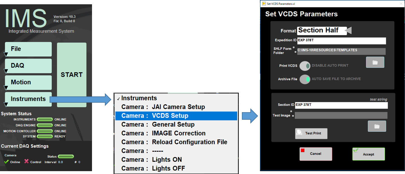
Figure 60. Select VCDS Setup
Several configurable options appear:
- Format: Choose between Side by Side or Section Half scratch pages.
- Expedition ID: Enter the name of the Current Expedition. This prints on the scratch sheet.
- SHLF Form Folder: Currently hard-coded to C:\IMS10\RESOURCES\VCD-S_TEMPLATE.
- Print VCDS: Enables or disables automatic printing of the scratch sheet. When the button says 'enable auto print' scratch sheets will automatically print when an image is saved.
- Archive File: Button enables disables saving scratch pages to the hard drive. All files are saved in .PNG format. If button says 'Do not save file to archive' files will not be saved.
- Section ID: Insert your expeditions name here which will appear in the top right corner of every scratch sheet along with the Text ID of the section half.
- Test Image and Test Print: Allows prints of images already on the computer or in the database to see the scratch sheet. Use the folder icon to the right of 'Test Image' to browse to a section half image of your choice. This image will be embedded into your chosen scratch page mode. Click the 'Test Print' button to send it to the printer.
- Accept: Saves any modifications to parameters.
Cancel: Does not save parameter modifications and reverts back to prior settings.
Editing Scratch Sheet in LabVIEW
- Navigate to C: > IMS-10 > Resources > Templates and double-click a VI to open it in LabVIEW.
- The front panel will open. Edits can be made to the objects on the white space. Editing the white or gray areas could affect scaling of the image, ruler, or print layout
- The main layout consists of an outermost borderless white box that indicates the printable area that is available.
- The leftmost gray column is a control for the section-half image and the ruler; do not make alterations in this area. There are two additional controls that feed the scratch page titles on the top left and right sides. These are not immediately visible when editing the layout on the front panel though. If you are not very familiar with LabVIEW please see a developer for help. The title controls can be moved, but it is up to you to remember where you put them!
All other column widths and headers are available for editing/resizing. If you need more columns simply select one, then copy/paste as you would in any standard graphics program and resize things to fit within the outermost white box. Maintain the vertical scaling of all columns to match that of the ruler/image column on the left. Header blocks are just boxes that can be copied and resized as well.
How to Make Edits
Navigate to the 'View' button on the toolbar. Select the 'Tools Palette' Option (Figure 61).
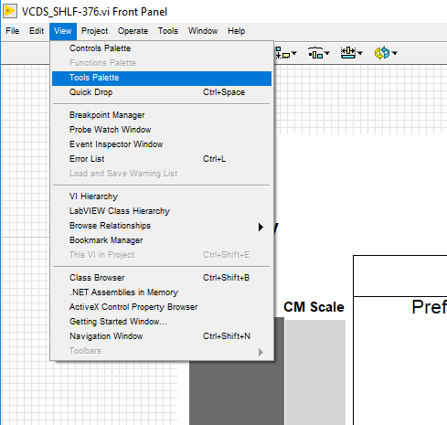
Figure 61. Select Tools Palette on LabVIEW
2. The Tools Palette window will appear (Figure 67). This allows you to select objects.
Figure 67. Tools Palette window
VI. Credits
All improvements to the Quick Start Guides and User Guides are a communal effort, with honorable mention to the group of LOs, ALOs, and technicians who have helped.
VII. Archived Versions
SHIL User Guide - 27Sept2022
LMUG-SHILUserGuide-020320-1516-374.pdf
1 Comment
Unknown User (25dbb4e563432e130164eb68f519000c)
Reviewed by Nicolette 6 August 2018
Areas in red need to addressed.