Table of Contents
I. Introduction
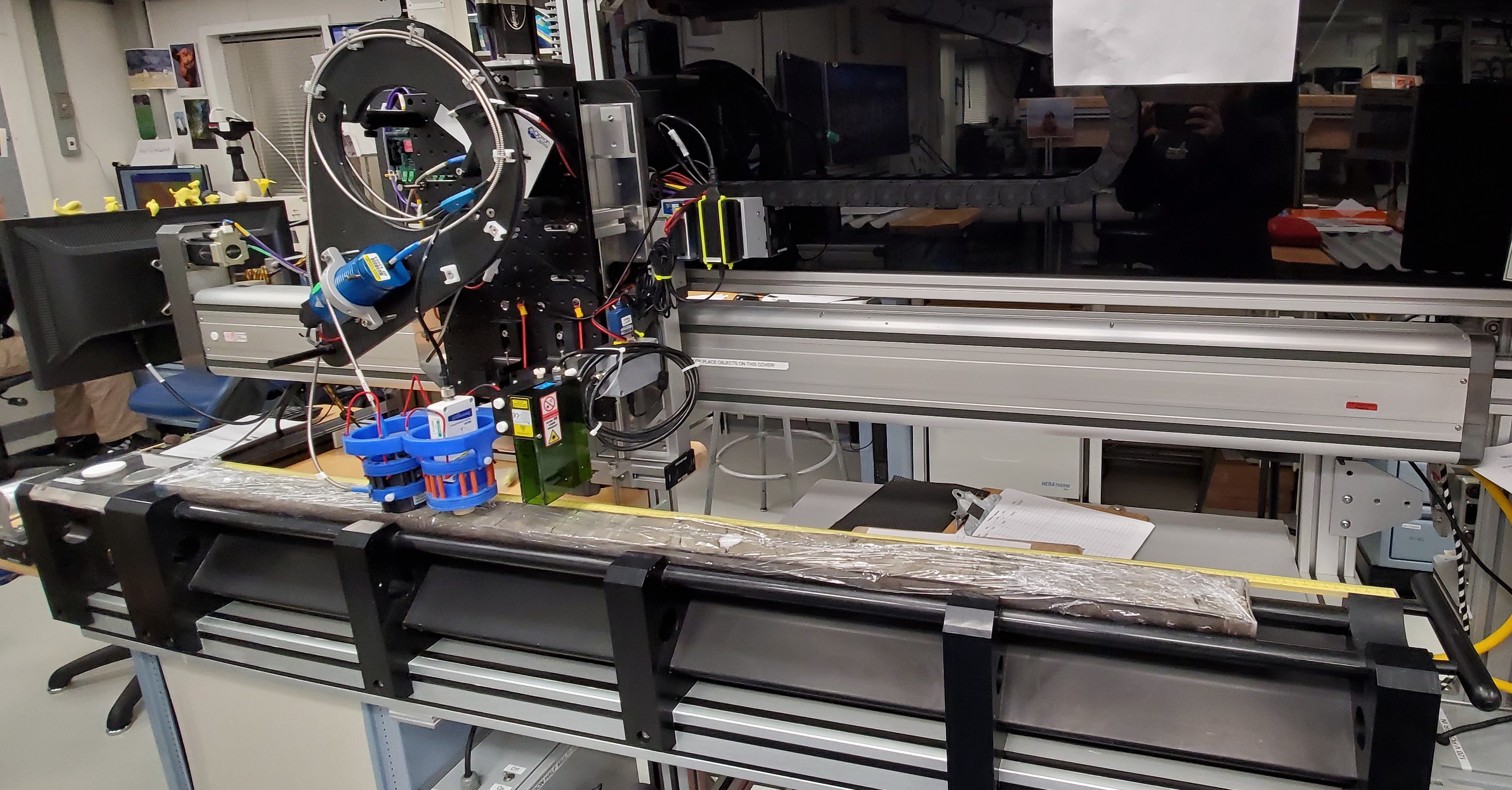
The Section Half Multisensor Core Logger succeeded the Archive-Half Multisensor Track (AMST) in the physical properties laboratory. The SHMSL simultaneously measures spectral reflectance and magnetic susceptibility on core section halves. Data generated from these sensors are used to augment the core descriptions.
Reflectance Spectrometry
–Percent reflectance plotted against depth supports lithology descriptions.
–Color parameters can provide a detailed time series of relative changes in the composition of the core material and can be used to correlate sections from core to core or hole to hole and to analyze cyclicity of lithologic changes.
–Spectral data can be used to estimate the abundances of certain compounds.
- Visible range provides semiquantitative estimates of hematite and goethite with better sensitivity than XRD.
- Near-infrared or near-ultraviolet ranges allow estimates of carbonate, opal, organic matter, chlorite, and some combinations of clay minerals.
Magnetic Susceptibility
Magnetic Susceptibility can be used to confirm whole-round core section magnetic susceptibility measurements. The SHMSL can measure magnetic susceptibility at a similar sampling point spacing to the whole-round measurements, or the user can select a completely different frequency of analysis.
MS data is used for correlation with other age-depth proxy measurements.
Theory of Operation
A split and scraped core section in a half-core liner is placed on the core track, where a barcode scanner is used to scan the section ID (from the end cap) and imports sample information from the LIMS. The electronics platform moves along a track above the core section, recording the sample height in the core liner using a laser sensor. The laser establishes the location of bottom of the section. When this step is finished, the track will pull up out of the way of the user in order to facilitate the covering of the core section with GLAD® Plastic Wrap. When the user covers the core section and answers the prompt, the platform reverses the direction of movement, moving from bottom to top while recording point magnetic susceptibility and spectral reflectance data at user-specified data acquisition intervals (generally 2–10 cm).
Reflectance Spectrometry
–Measured from 380 to 900 nm at 2 nm intervals using both an LED and a halogen light source, covering a wavelength range through the visible spectrum and slightly into the infrared domain. Currently only 390nm to 732nm is being recorded. Waiting to hear back from Bill Mills.
–Scanning the entire wavelength range takes ~5 s per data acquisition offset.
–Data are generated using the CIELAB L*a*b* color system:
- L* represents lightness, where 0 yields black and 100 indicates diffuse white;
- a* represents magenta to green tinting, where negative numbers indicate red/magenta shading and positive numbers indicate green shading; and
- b* represents yellow to blue tinting, where negative numbers indicate yellow shading and positive number indicate blue shading.
–Data are also stored and returned as CIELAB Tristimulus XYZ values. The definition of X, Y, and Z is complex and the reader should refer to reference materials for an explanation. Refer to the related documentation section below.
–Finally data are stored and returned as RGB values to facilitate comparison with the imaging logger RGB values; note however that the sampling interval is quite different between the imaging logger and the integration sphere.
Magnetic Susceptibility
–Measured at the same data acquisition rate as spectral reflectance using a contact probe with a flat 15 mm diameter sensor.
–The sensor can be configured for different integration times (1 Hz or 0.1 Hz) and different numbers of replicate measurements. Our standard conditions are 3 measurements at 1 Hz measurement frequency for each offset. These three results are averaged and uploaded to the database. Thermal drift is effectively eliminated by zeroing the meter before each section.
–Data are reported in dimensionless instrument units (SI). In order to use these data as SI magnetic susceptibility units, the appropriate volume correction must be applied, which varies by sensor type. The user should not use the cgs setting so that the data set is consistent with previous measurements and with the whole-round logger results.
II. Procedures
A. Preparing the Instrument
- Double-click the MUT icon on the desktop (Figure 1a) and login using ship credentials. For more information on data uploading see the "Uploading Data to LIMS" section below.
- Double-click the IMS icon (Figure 1b). IMS initializes the instrument. Once initialized, the logger is ready to measure the first section.
![]() Figure 1. (a) MUT Icon. (b) IMS Icon.
Figure 1. (a) MUT Icon. (b) IMS Icon.
At launch, the program begins the following initialization process:
- Tests all instrument communications
- Reloads configuration values
- Homes the X and Y axis
After successful initialization, the main IMS- SHMSL window will appear (Figure 2).

Figure 2. IMS Application Main Screen.
The IMS Control panel (Figure 3): Provides access to utilities/editors via drop-down menus.
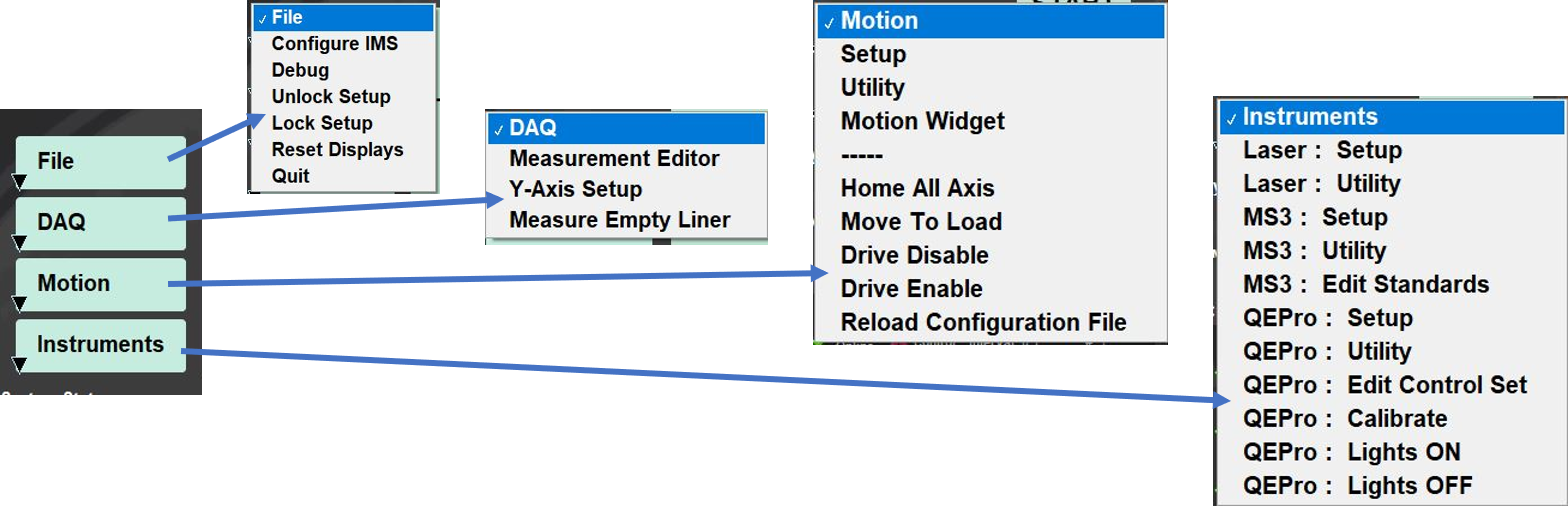
Figure 3. Control Panel Drop Down menus.
START button will allow the user to begin measurements. Section Information window (Figure 4) will pop up.
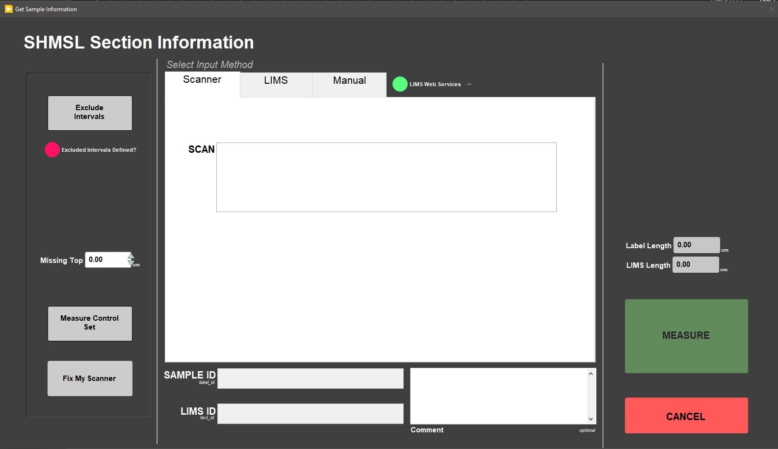
Figure 4. Section Information window.
Prior to measuring a section half on the SHMSL, the user must:
- Calibrate the QE Pro Spectrophotometer
- Set the measurement interval for each instrument.
B. Instrument Calibration
a) Color Reflectance Spectrophotometer
The color reflectance spectrophotometer calibrates on a spectra, pure white (Spectralon® WHITE standard) (See Important Notes for further information), and the black is acquired with the lights off and the shutters, but closed still on the white Spectralon standard. The spectrometer calibration can be triggered automatically (typically every 6 hours) or manually by the user. The expiration time for the spectrometer calibration is set in the QEPro setup menu (Figure 16). Before running the first sample, the software will check the status of the spectrometer calibration. If the calibration has expired, a prompt will appear asking the user to begin an automatic calibration (Figure 5). It is recommended that the user calibrate every time the software prompts the user.
There is an option to ignore the calibration, but the calibration prompt will reappear with every run until the calibrations are completed. Data run without a calibration update will be flagged as calibration invalid in LIMS.
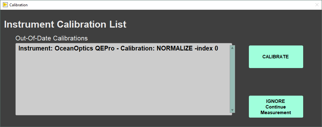
Figure 5. Instrument Calibration Prompt
Automatic Calibration
1. Before beginning the calibration, ensure the WHITE standard is clean (Figure 6). If the Spectralon® standard appears even the least bit gray or discolored, contact the technician to clean or replace the standard! It may be useful to compare a clean, new piece of white paper to the standard—if the paper seems whiter, the standard is quite dirty.
a. The Spectralon® standard can be cleaned according to the Spectralon® Reflectance Standards Care and Handling Guidelines. Spectralon Standards Care and Handling.pdf. Check that both lights are on and the shutters are open. If you look at the white standard while the integrating sphere is over it you should see two dots of light, one blue (LED) and one yellowish (Halogen).
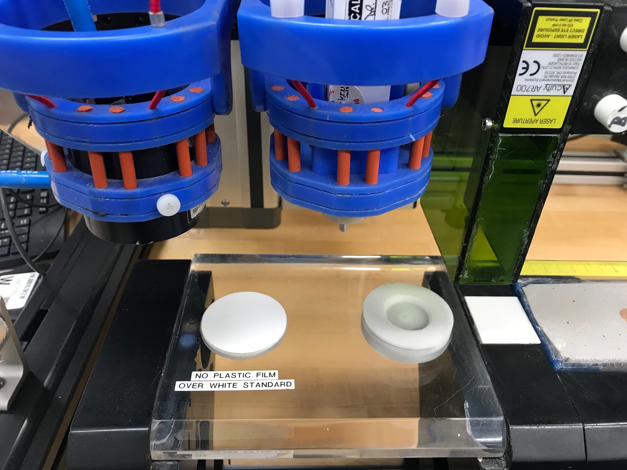
Figure 6. White color reflectance standard calibration (left) and MS standard (right).
2. Click the CALIBRATE button to begin the calibration process. The user may select IGNORE Continue Measurement and skip the calibration, but the software will prompt the user for a calibration every time a measurement is started until the calibration is completed.
a. The logger moves the QE Pro integrating sphere over the WHITE calibration standard and lowers the sensor until it touches. The sensor begins the white calibration measurements (Figure 7) based on the set saturation level of the total response (Review Setup parameters window).
b. The display includes:
- Max Counts: current highest value
- Target Counts: percent saturation value as set in the instrument parameters (range = 32,000 counts)
- Integration Time: measurement period where the highest wavelength count is equal to or exceeds 80 percent of the spectrophotometer's range.
3. When the white calibration is complete, the integration time will be displayed on the screen and the user will be prompted to Accept, Re-Start, or Abort the calibration (Figure 8).
a. The integration time should be about 0.30 to 0.55 seconds for the current dual-light source configuration, assuming the bulbs are new.
b. If integration times increase to more than 1 second, alert the IODP technician. The halogen bulb or the LED source may need replacing.
4. Click Accept to accept the white calibration.
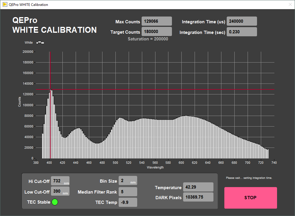
Figure 7. White Calibration Screen
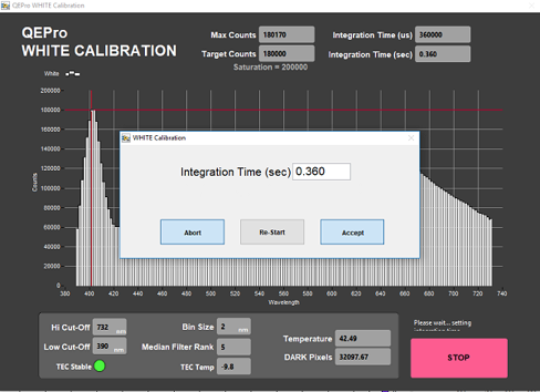
Figure 8. White Calibration Integration Time Display
5. After the WHITE measurements are completed, the shutters on the light sources will close and the DARK measurement will acquire 20 measurements. The dark measurement is a baseline measurement that includes thermal noise of the system. On the screen (Figure 9):
- Temperature: should remain below 50°C; note that the TEC temperature is usually about -9 degrees C; accessed through the QE Pro Utilities screen.
- Spectral Mean: mean of the entire spectrum (at the line across the display plot). This should be only about 200 counts higher than the Dark Pixel count. With plastic wrap, it should not exceed 500 counts
- Dark Pixels: 20 pixels that have been deliberately masked to allow no light. These counts represent the thermal noise of the spectrophotometer.
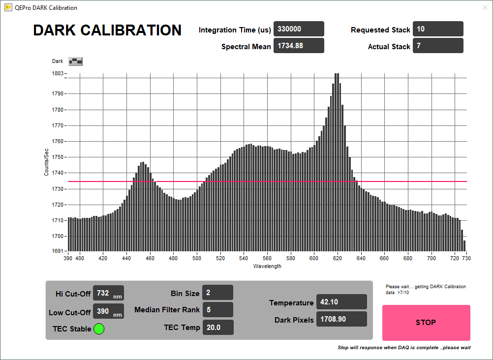
Figure 9. DARK Calibration Screen
6. When the dark calibration is complete, the user is prompted to Abort, Re-Start, or Accept the dark calibration (Figure 10).
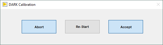
Figure 10. Dark Calibration Completed Prompt
7. The final screen shows the normalization of spectra that will occur with the just-acquired calibration (note: low values are better than high values because of signal-to-noise ratio) (Figure 11). Ideally, the graph would display a straight line at zero value. However, a normalization factor is required to be applied to the XYZ and L*a*b* color indexes. Normalization amplifies the noise as well as the signal. If core flow allows, the data quality can be increased by averaging multiple measurements (in Measurement Editor increase the Average parameter).

Figure 11. Calibration Normalization Factor
8. Select Accept. If this was an automatic calibration at the start of a measurement, the laser profile will start automatically, followed by the normal measurement sequence.
Manual Calibration
To perform calibration manually (not when specified by the software), select Instruments > QE Pro: Calibrate (Figure 3). The QEPro will move to the white standard and begin the calibration process. Follow the automatic procedure from step 4 to complete the calibration. This should be performed when a bulb is changed or other hardware configuration changes.
Recognizing a Bad Calibration
The following information is provided to assist scientists and technicians in evaluating the QE Pro calibration. Always verify the lights are on and the shutters are open. Two dots of light should be visible exiting the integration sphere.
- Figure 12, demonstrates a calibration with an old light source. When the 500nm - 740nm end of the calibration spectrum is over the amount of counts the program will process, this might be for a number of reasons, but most likely the LED light is dim or off. The blue end of the spectrum is within the correct amount of counts and maintains the right curve with the spike around 400 wavelength and a dip into the 420-430 range. The first thing to check is the age of the LED light source, if it is older than 1 month it should be replaced.

- Figure 13 demonstrates a calibration with the LED turned off (i.e., the shutter did not close properly). You'll notice the left side of the graph, the blue side, does not show the proper peaks, whereas the red side of the graph is at 180K counts. Make sure the LED light is in TTL mode and properly connected to the QE Pro, and lastly that the shutter is opening. If you look at the white standard while the integrating sphere is over it you should see two dots of light, one blue (LED) and one yellowish (Halogen).
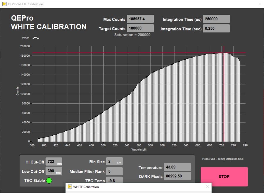
Figure 13 - White calibration, blue light (LED) turned off or other malfunction.
Measuring the Color Control Set
There are twelve color reflectance standards available in the physical properties lab in the drawers beneath the pycnometer. The black standard is not typically used in the control set.
Measuring the Control Set:
- Set the standard holder on the track as seen in Figure 14.
- The standard holder has a white block on one end. This white block should be against the white benchmark on the track for proper positioning (Figure 14, red circle).
- Place the color standards in the sample holder.
- The order and position of the standards are set under the Instruments > QE Pro: Edit Standards menu. See the Utilities: QEPro Edit Control Set section for more information about setting up the control set.
- Select Start from the main IMS window (Figure 2).
- Select Measure Control Set.
- The QE Pro will begin moving down the track and collecting measurements on each standard. The data for each standard will be displayed on the screen (Figure 15).
- . If the QE Pro does not properly touch down on the standards, the positions may need to be edited in the Instruments > QE Pro: Edit Standards. Also verify that the standard holder is against the benchmark.
- After each standard has been measured, the data will automatically be saved to the C:/AUX_DATA/RSC/CNTRL folder as a .csv
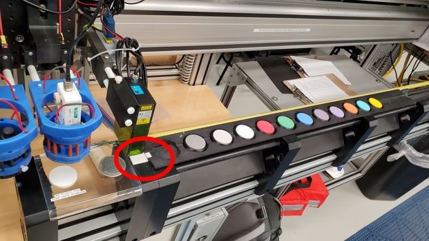
Figure 14. Color Reflectance Control Set on SHMSL track. The white square on the end of the standard holder should be against the white benchmark (red circle).
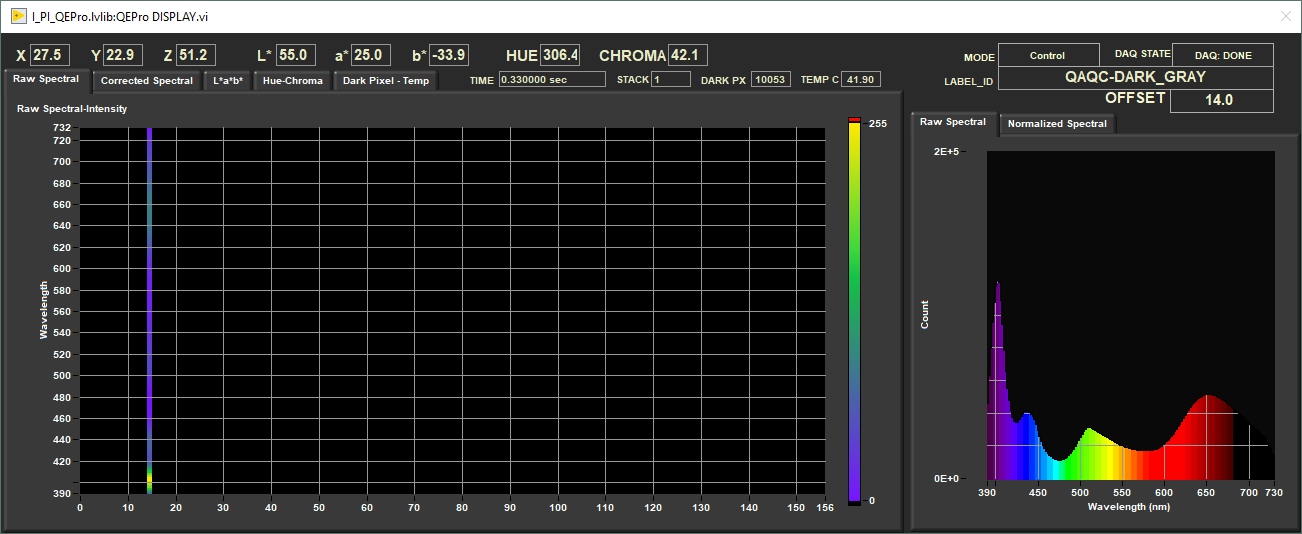
Figure 15 - IMS-SHMSL Display during control set measurements
b) Magnetic Susceptibility Meter
The point magnetic susceptibility meter is calibrated by the manufacturer (Bartington, Ltd.). The probe is zeroed in air before the core section is measured, so drift is not a significant factor. It is not necessary to calibrate the MS2K or MS2E probes (or the MS2C loops on the whole-round loggers), but the calibration check standard can be used to demonstrate consistent results.
C. Set Measurement Parameters
a) Instrument Setup
Each instrument has a separate setup menu. Configuration values should be set during initial setup by the technician and scientists. The general instrument setup should not change unless there have been changes to the hardware.
QEPro Configuration
Select Instruments> QEPro: Setup (Figure 3). The QEPro Parameters window will open (Figure 16). This window is divided into 4 sections: General Setup, Acquisition Parameters, White and Dark Standards, and Integration Time.
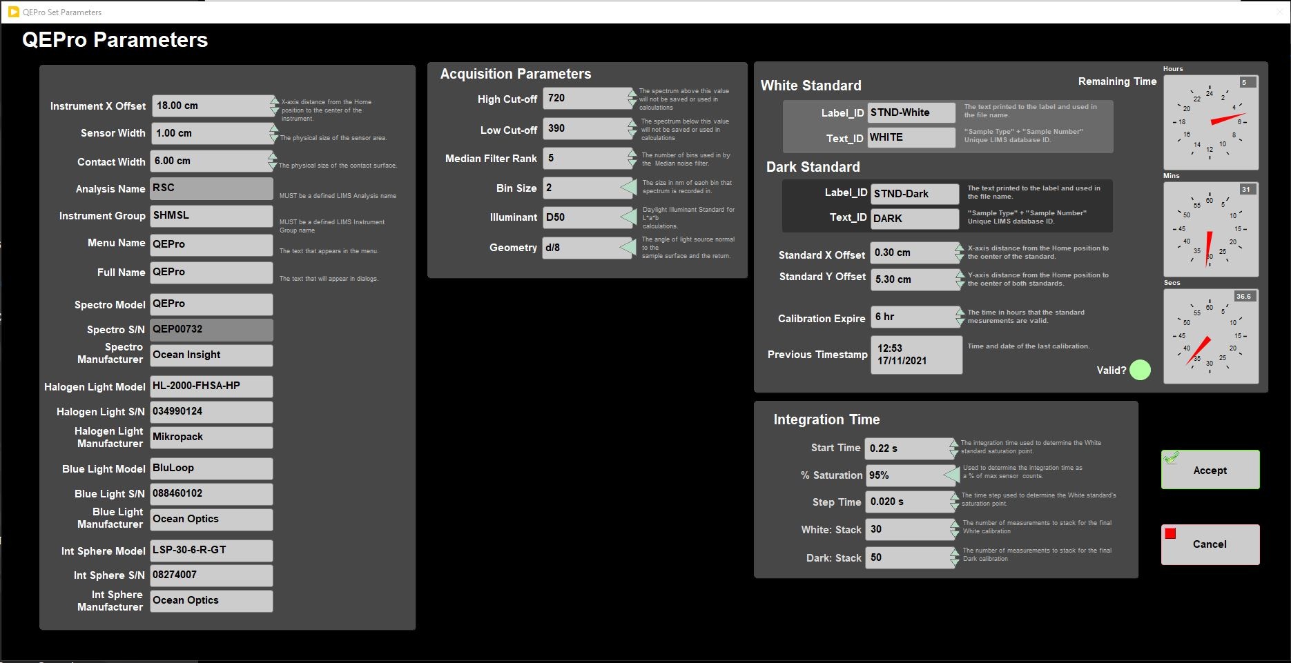
Figure16. QEPro Setup Window
General Setup
- Instrument X offset: The x-axis distance of the laser where the center of the sensor is over the benchmarks zero edge.
- Sensor Width: Physical size of the sensor area
- Contact Width: Physical size of the contact surface
- Analysis name: LIMS analysis component (must match LIMS component exactly).
- Instrument group: LIMS instrument group logger name (i.e., SHMSL).
- Model: Model name of the sensor (from manufacturer).
- S/N: Serial number of the sensor (from manufacturer).
- Manufacturer's Name: Name of the manufacturer of the QEPro spectrometer.
- Menu name: value that appears as the instrument's menu name.
- Full name: value that appears in instrument dialog boxes.
Acquisition Parameters section
High Cut-off: Used to define the upper limit of the region of interest (ROI) in the spectrum. The spectrum above this value will not be saved or used in calculations. (Figure 17)
- Low Cut-off: Used to define the lower limit of the region of interest (ROI) in the spectrum. The spectrum below this value will not be saved or used in calculations. (Figure 17)
- Median Filter Rank: Number of adjacent channels used to filter noise from the signal.
- Bin size: The width (nm) of each bin that the spectrum is recorded in. (Figure 17)
- Illuminant: The Daylight Illuminant Standard for L*a*b calculations; International Commission on Illumination (CIE) standard illuminant used in color calculations (also called daylight illuminant)
- Geometry: References integration sphere measurement technique: illumination from a diffuse light source viewed 8° from normal (d/8); includes a gloss trap to exclude spectral reflections.
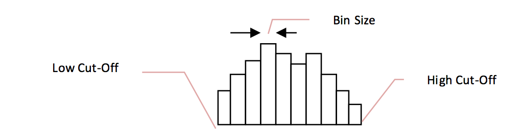
Figure 17. Illustration of high and low cut-off and bin size.
White and Dark calibration Section
- White Label ID: LIMS label_ID component value (STND-White).
- White Text ID: LIMS text_ID component value (WHITE).
- Dark Label ID name: LIMS label_ID component value (STND-Dark).
- Dark Text ID: LIMS text_ID component value (DARK).
- Standard X-offset: Track position (X-axis; in cm) of laser when the center of the integration sphere sensor is over the center of the white standard.
- Standard Y-offset:Llift position (Y-axis) when the integration sphere is in contact with the White or Dark standard (same value for both).
- Calibration expire: Time in hours between calibrations. The user will be given a warning when the calibration time has expired.
- Previous Timestamp: Time and date of last calibration (read only).
- Remaining time: Clock displays of the time remaining until the next calibration is needed (read only).
Integration time section
- Start Time: The integration time used to determine the white standard saturation point
- % Saturation: Used by WHITE calibration to determine sample integration time by calculating the integration time required to reach the specified saturation (70%–95%). Note: if cores are light colored, increase throughout by using a low saturation level; if cores are dark colored, use a high saturation level to improve signal-to-noise ratio.
- Step Time: The time step used to determine the White Standard's saturation point
- White: Stack: The number of measurements to stack for the final White calibration
- Dark: Stack: The number of measurements to stack for the final Dark calibration
MS3 Configuration
Select Instruments> MS3: Setup (Figure 3). The QEPro Parameters window will open (Figure 18). This window is divided into 3 sections: General Setup, MS Correction Factor, and Select MS Control
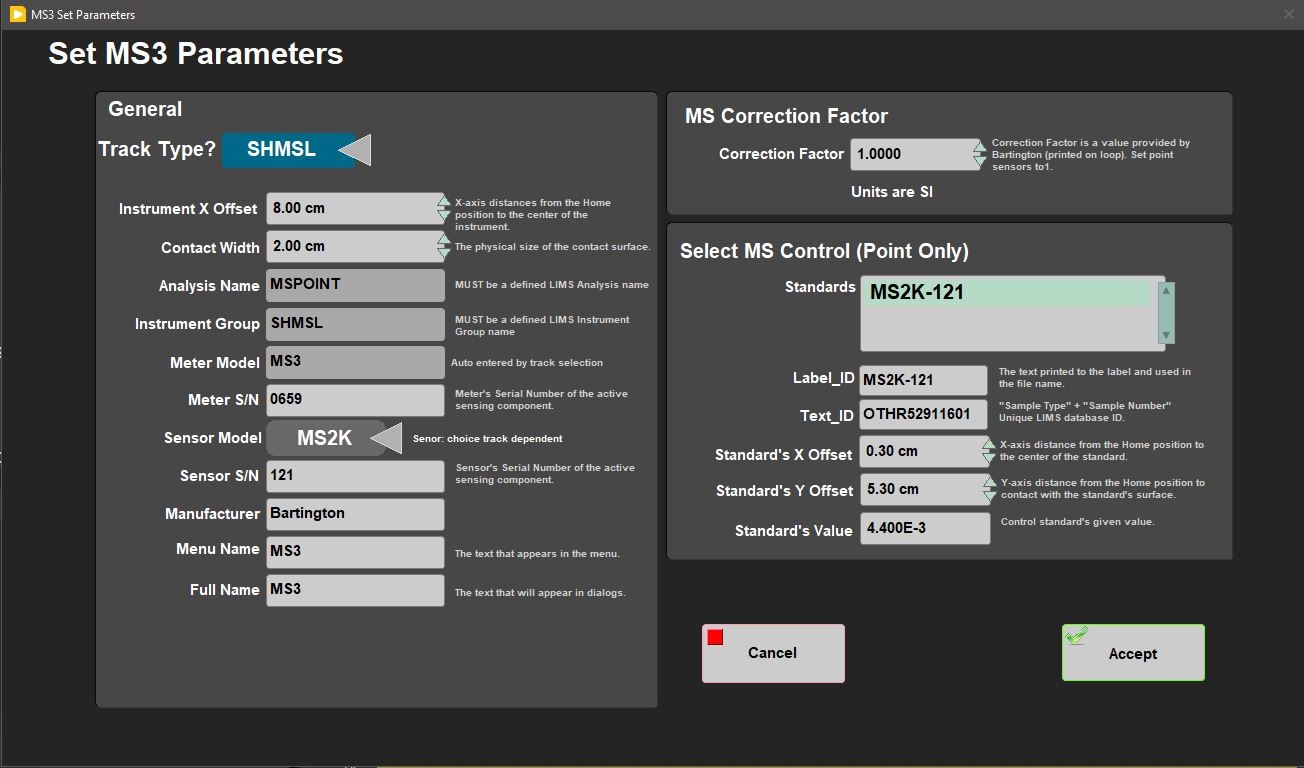
Figure 18: MS2 Setup Window.
General Setup
- Track and Sensor Type: Select the type of MS sensor and the track (SHMSL- Point)
- Instrument X Offset: The x-axis distance to the sensor, where the center of the sensor is over the benchmarks zero edge
- Contact Width: Physical size of the contact surface
- Analysis name: LIMS analysis component (must match LIMS component exactly).
- Instrument group: LIMS instrument group logger name (i.e., SHMSL).
- Meter Model: Model name of the sensor (from manufacturer).
- Meter S/N: Serial number of the sensor (from manufacturer).
- Sensor Model: Sensor's Model of the active sensing component.
- Sensor S/N: Sensor's Serial Number of the active sensing component.
- Manufacturer's Name: The name of the manufacturer of the MS sensor
- Menu name: Value that appears as the instrument's menu name.
- Full name: Value that appears in instrument dialog boxes.
MS Correction Factor
These values are used when attempting to match data between multiple sensors. Default values are 1.
- Correction Factor: A correction factor provided by the Bartington. Typically 1.
- For standard-frequency loops (80 and 90 mm, 565 Hz), this value is 1.000.
- For 10% high loops (80 mm only, 621 Hz), this value is 0.908.
- For 10% low loops (80 mm only, 513 Hz), this value is 1.099.
- For 20% low loops (90 mm only, 452 Hz), this value is 1.174.
Select MS Control (Point Only)
- Standards: Name of the standard being used.
- Label ID: The label ID used to identify the standard.
- Text ID: Unique identifier for the standard in the database.
- Standard's X offset: Track position (X-axis) of the laser when the center of the MS sensor probe is over the center of the standard.
- Standard's Y offset: Lift position (Y-axis) when the MS sensor probe is in contact with the standard.
- Standard's Value: The standard's accepted/given value. Value established by IODP is 48 +/- 2 SI.
Laser Configuration
Select Instruments> Laser: Setup (Figure 3). The AR700 Parameters window will open (Figure 19).
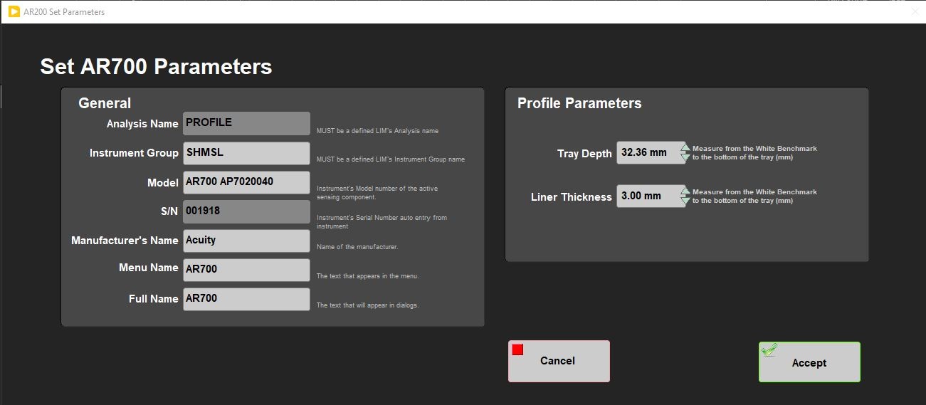
Figure 19: AR700 Setup Window
General Setup
- Analysis name: LIMS analysis component (must match LIMS component exactly).
- Instrument group: LIMS instrument group logger name (i.e., SHMSL).
- Model: model name of the sensor (from manufacturer).
- S/N: serial number of the sensor (from manufacturer).
- Manufacturer's Name: The name of the manufacturer of the laser.
- Menu Name: Laser
- Full name: value that appears in instrument dialog boxes.
Profile Parameters
- Tray Depth: Measure from the White Benchmanrk to the bottom of the tray (mm)
- Liner Thickness: Measure from the White Benchmark to the bottom of the tray (mm)
b) Set Measurement Parameters
The user may adjust the measurement parameters for each instrument on the SHMSL by selecting DAQ> Measurement Editor (Figure 3). The measurement editor window will open (Figure 20).
To edit the settings for a particular instrument, select the instrument from the list on the left side of the window and then click within the Instrument Parameters block on the right side of the screen. A window, like in Figure 21, will open.
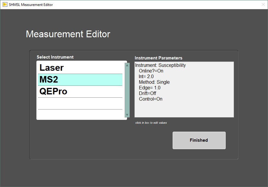
Figure 20. Main Measurement Editor Window
QE Pro Measurement Parameters
Settings available in the QE Pro Measurement editor (Figure 21) include:
- Interval: The measurement interval in centimeters.
- Edge: The interval of core to exclude at the start and end of a section and at the edges of gaps in the core.
- Method: Select to take a single measurement at the time set by the white calibration or to stack multiple measures and average using the measurement time set by the white calibration.
- Stack: The number of measurements to average at a given position.
- Control: Control ON will measure the white standard as a control each time a section is measured.
- Online?: Suspend measurements with the QE Pro.
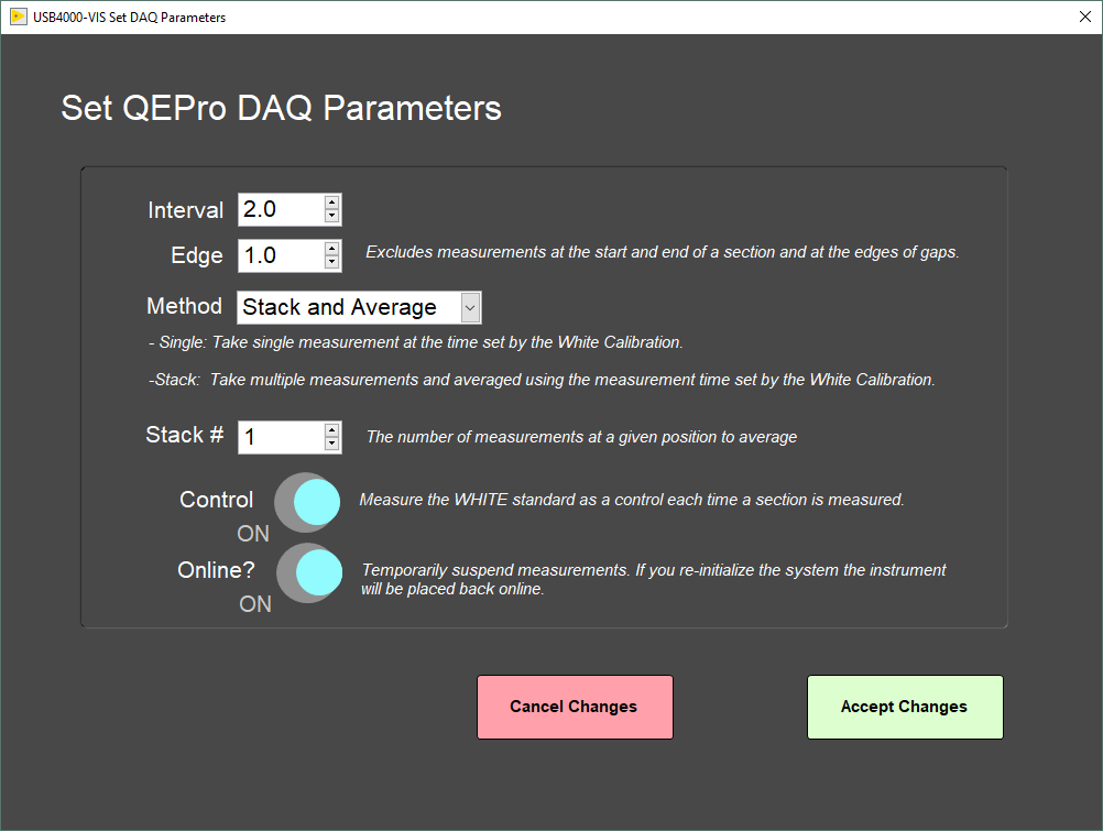
Figure 21. QE Pro Measurement Parameters.
MS Measurement Parameters
Settings available in the MS3 Measurement editor (Figure 22) include:
- Interval: The measurement interval in centimeters.
- Edge: The interval of core to exclude at the start and end of a section and at the edges of gaps in the core.
- Meas. Time: Integration time used for a measurement.
- Zero Meas. Time: Integration Time used for zeroing the meter (air blank).
- Control: Control ON will measure the MS standard as a control each time a section is measured
- Online?: Suspend measurements with the MS point sensor
- Drift Correction: Applies a two-point drift correction to the data. A measurement is taken before the laser profile and another after measuring the standard, at the end of the test.
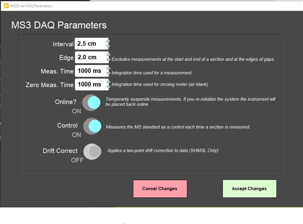
Figure 22. MS3 Measurement Parameters.
Laser Measurement Parameters
The user may use the Laser Measurement editor (Figure 23) to set the gap offset. This is the height below the benchmark which will be tagged by the system as a gap and will therefore not be measured. For piston cores, the recommended gap offset should be set to 10 mm to 13 mm. For hard rock cores, the gap offset should be set between 20 and 30 mm.
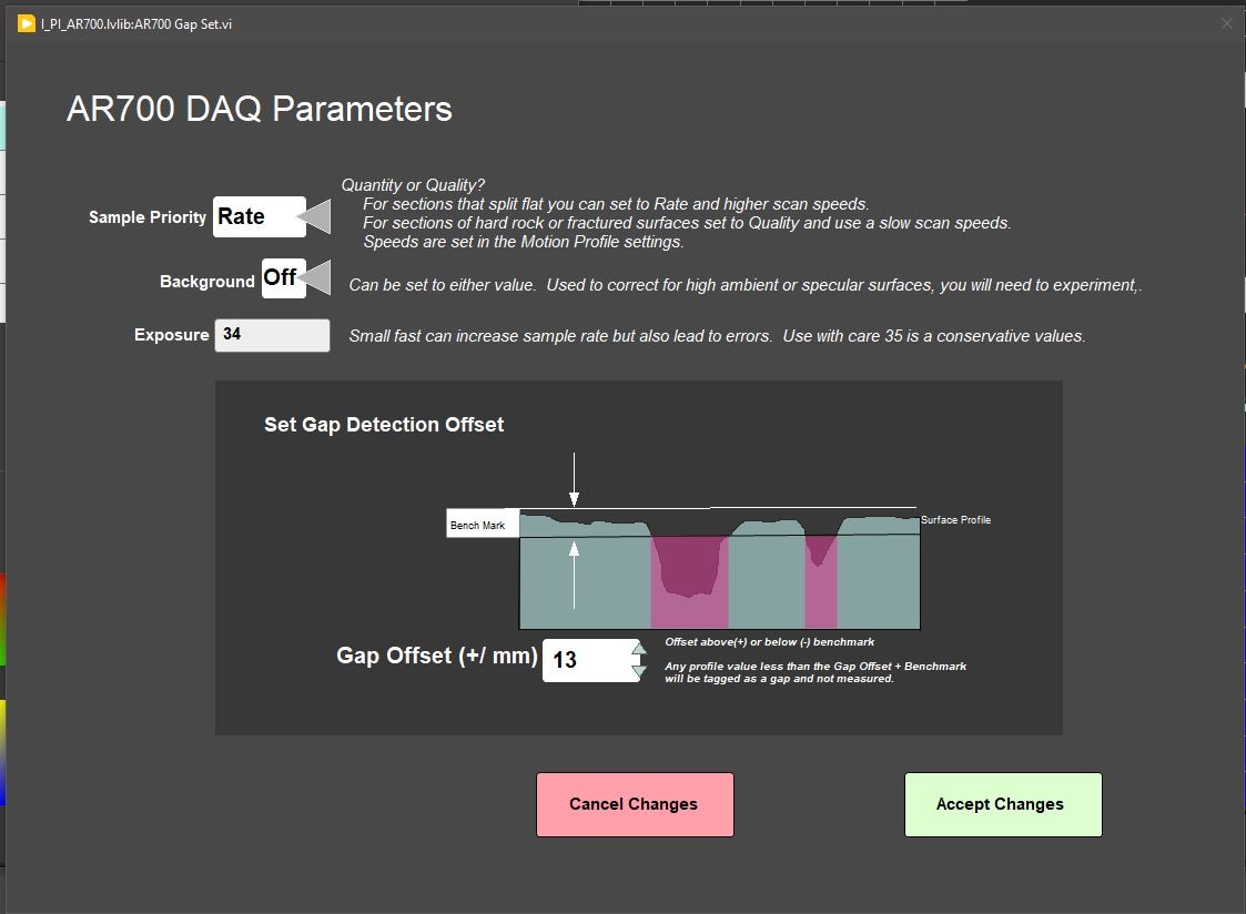
Figure 23. Laser Measurement Parameters
D. Preparing Sections
- Use a spatula or smear slide to clean the cut surface of the core by lightly scraping away any material that was smeared across the surface during core splitting. Take the SHIL and X-Ray image first so SHMSL sensor footprints will not be in the image.
- Bring the endcap of the section half (usually A for archive half) to be measured to the SHMSL, you will use the endcap to scan the barcode for sample information.
- Place the archive section in the core tray with the blue endcap up against the benchmark. The benchmark is the white square at the head of the rails that hold the section halves (Figure 24). If material is missing at the top of the section, section half should be positioned all the way up to the top of the rail.
- Adjust the section so that it is as flat as possible with respect to the plane of the benchmark. There is a limit to how much the sensor heads can float when they land on a tilted section.
- Do not wrap the cores yet. The Acuity AR700 laser cannot reliably see through the plastic to measure an accurate profile of the section half surface.
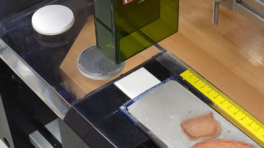
Figure 24. Benchmark location
Note: This analysis requires clear polyethylene film such as GLAD® Wrap. Other types of plastic wrap will not serve.
E. Making a Measurement
- Select Start from the main IMS SHMSL window (Figure 2). The SHMSL Section Information window will open (Figure 4).
2. Place the cursor in the SCAN text field (Figure 4) so that the barcode information will be parsed appropriately. Scan the section label on the section half end cap.
- The Sample ID, LIMS ID and LIMS length will automatically parse.
- User also has the option to use the LIMS entry tab or the manual entry tab for entering sample information. Be aware that samples must be named properly when using the Manual tab or the data files will not be uploaded to LIMS.
3. Additional features are available in the Sample Information window. These include:
- Exclude Intervals: Intervals can be specified for omission (Figure 25). Enter the top and bottom offsets of the areas to be excluded during the measurement. The excluded intervals apply to all enabled sensors. A green indicator on the sample information entry window (Figure 4) will appear when intervals are set to be excluded.
- Exclude Intervals: Intervals can be specified for omission (Figure 25). Enter the top and bottom offsets of the areas to be excluded during the measurement. The excluded intervals apply to all enabled sensors. A green indicator on the sample information entry window (Figure 4) will appear when intervals are set to be excluded.
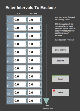
Figure 25. Exclude Intervals Window
- Missing Top: When the top of the section is missing, typically due to whole round sampling, the value, in centimeters, of missing material can be entered into the Missing Top field. The software will calculate the measurement offsets based off this entry.
- Fix My Scanner: Use this feature to reprogram the barcode scanner to properly parse section half labels for use with the SHMSL software.
- Measure Control Set: This feature is used to trigger the QE Pro to measure the color reflectance standards. See the Measure Control Set section under Instrument Calibration.
4. Select Measure
- The sensor assembly will move down the track while the laser acquires a profile of the split surface of the section (Figure 26).
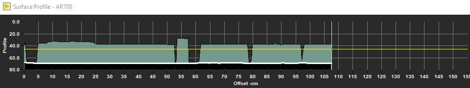
Figure 26. Laser Profile
b. When the software has detected a gap, it will indicate regions that will not be measured by the MS and reflectance sensors on the screen in red.
Note: (Gap detection parameters are configurable in the DAQ> Measurement Editor Laser window (Figure 23).
c. The laser looks for a gap deeper than the average section-half thickness. If end of section is on one of the bench blocks, the end of section may not be detected accurately.
5. When the laser reaches the end of the section, the Section Length confirmation window will appear (Figure 27).
- Verify the section length, in centimeters, is correct. If the laser length is longer than the section, manually enter the correct length in the scan length field.

Figure 27. Section Length Confirmation Window
6. Apply GLAD® Plastic Wrap to the surface of sediment cores.
a. IMPORTANT!!! It is necessary to cover the core section with GLAD® PlasticWrap in order to avoid damage to the integration sphere. Any mud that gets inside the sphere will ruin it! Care should be taken to reduce wrinkles in the wrap.
b. IMPORTANT! Do not cover the standards with GLAD® Plastic Wrap; they will give erroneous results if you do.
7. Select Go. The measurement process will begin.
- For efficiency, measurements begin at the bottom of the section and move upcore.
- Results are displayed during acquisition on instrument graphs on screen. The QE Pro has several tabs that display different views of the color reflectance data (Figure 28). Tabs can be changed during the measurement sequence. The Corrected Spectra tab shows the corrected percent color reflectance being measured at each point.
- After the section has been measured, the logger takes measurements using the JRSO MS and WHITE standards as check standards, given that the control sample measurement was set up in the measurement parameters.
- For efficiency, measurements begin at the bottom of the section and move upcore.
6. When the measurements are complete, the instruments will return to home and the Sample Information window will be displayed. The user may now prepare the next section and continue measurements.
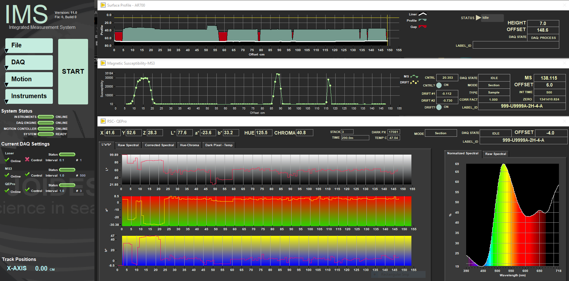
Figure 19. Main IMS- SHMSL Data Acquisition Display
F. Quality Assurance/Quality Control
Analytical Batch
The analytical batch is defined by the number of samples run between each spectrometer calibration. Each sample in the batch run with the current calibration is associated with that calibration data in the LIMS. If a calibration problem is discovered, all samples in the batch can be identified and rerun.
Accuracy
Magnetic Susceptibility
Measure a well-characterized magnetic susceptibility control sample and compare results with true value and/or whole-core track results.
Reflectance
Measure a second standard, standard reference material, or characterize a material in-house to use as a control. Measuring the BCRA-calibrated tiles ensures the desired accuracy is being maintained. This should be done periodically throughout each expedition.
Precision
Run samples or standard reference materials more than once (separate measurement runs) and calculate the standard deviation. This should be done every ~20-section halves allowing for a comparison between runs and estimation of uncertainty based on precision.
G. IMS Utilities
AR700 Utility
Select Instruments > Laser: Utility (Figure 3). The AR700 laser utility window will open (Figure 29). This utility allows the user to test the performance of the AR700 in real time and allows the user to ensure that the laser is returning true distance values.
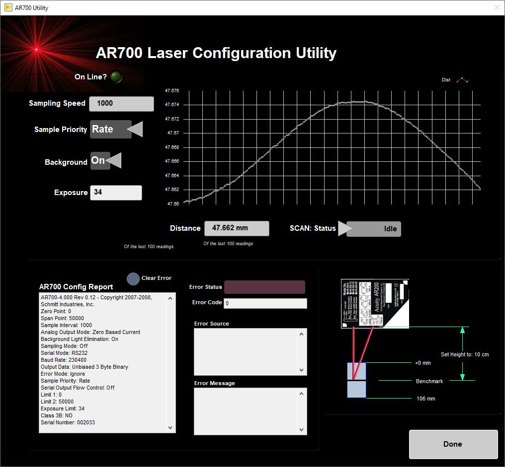
Figure 29. AR700 Laser Utility
Magnetic Susceptibility Utility
Select Instruments > MS3: Utility (Figure 3). The MS3 utility window will open (Figure 30). The utility allows the user to test the MS performance. The MS utility allows the user to zero the meter and to set it to continuous measurement.
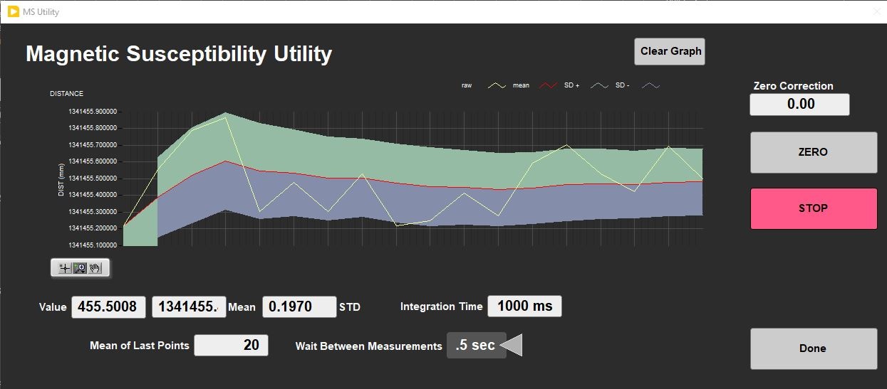
Figure 30. MS3 Utility
Magnetic Susceptibility Edit Standards
Select Instruments > MS3: Edit Standards (Figure 3). The Standard Set Editor window will be displayed (Figure 31).
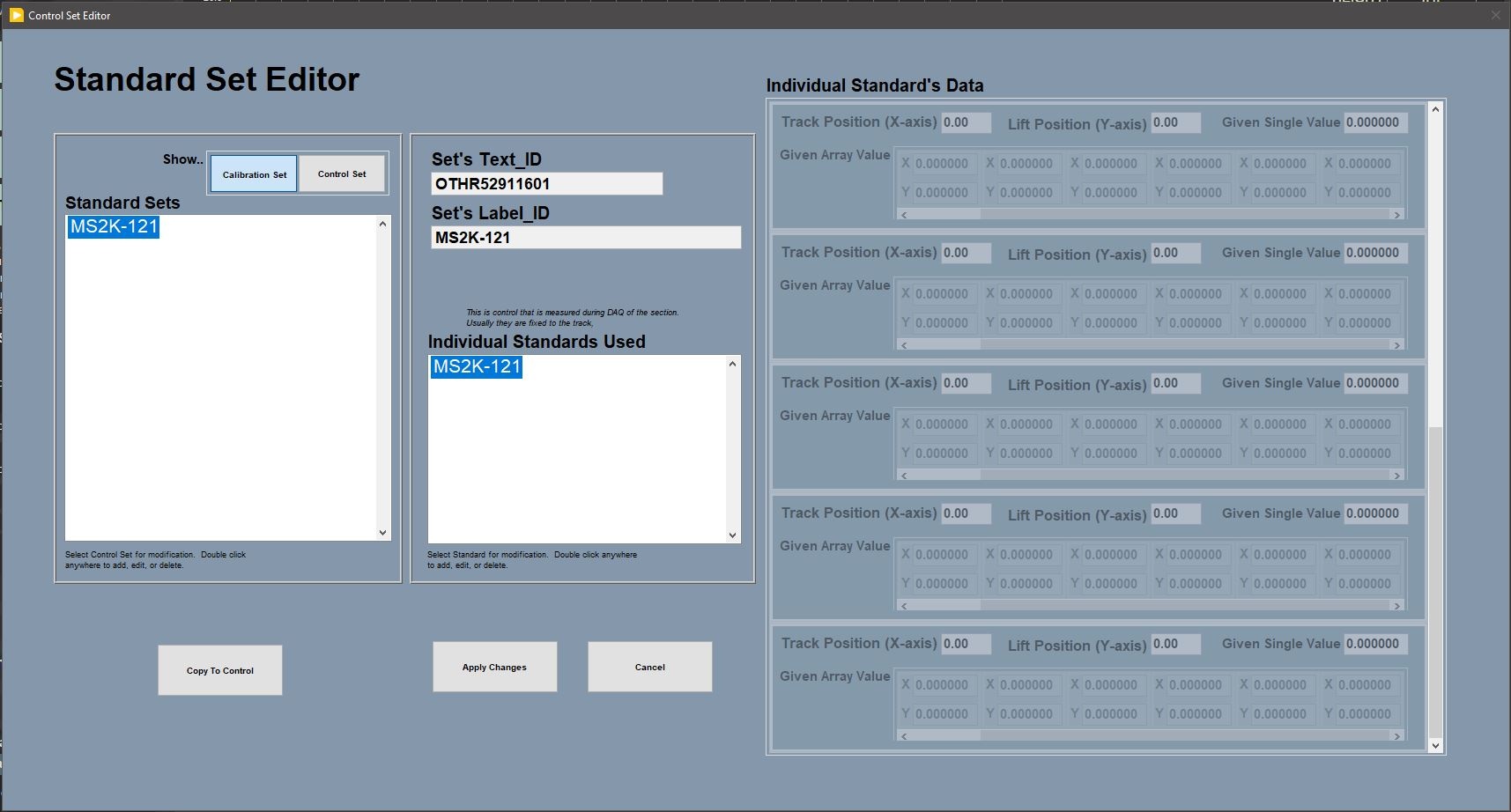
Figure 31. MS Standard Editor Window
QEPro Utility
Select Instruments > QEPro: Utility (Figure 3). The QE Pro utility window will open (Figure 32). The utility allows the user to run instantaneous or continuous measurements of the spectrum being acquired by the spectrometer. Different spectra (e.g., light standard, dark standard) can be overlaid and the user has a number of other options.

Figure 32. QE Pro Utility
QEPro Edit Control Set
Select Instruments > QEPro: Edit Control Set (Figure 3). The QE Pro Standard Set Editor window will open (Figure 33). This utility allows the user to define the standards and their positions on the track. These configuration values are used to determine where the QE Pro will be positioned for calibration measurements.
- To view the setup of the 99% white Spectralon® standard and the "dark" standard, select Show Calibration Set.
- To view the setup of the diffuse color standards, select Show Control Set.
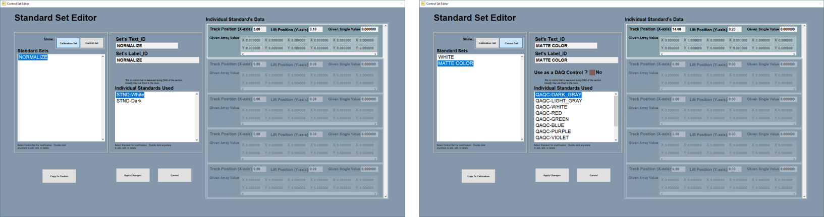
Figure 33. QEPro Control Set Window. The calibration standards can be edited (left) through the Calibration Set and the control set standards can be edited (right) through the Control Set window
To edit a standard:
- Select the standard of interest under the Individual Standards Used field
- The current configuration will be displayed under the Individual Standard's Data heading.
- Double click on the standard's name under the Individual Standard's Used heading. An action prompt will open (Figure 34).
- Select the Edit Standard option to update an existing standard's identification information or position on the track (Figure 35). Select New Standard to create a new individual standard.
- Scan the Standard Label into the Scanner field
- The standard labels can be found in Sample Master by selecting the Sample Table tab with the VIEW mode selected. The SHMSL standards will be listed under:
- Expedition:QAQC
- Site: CORELAB
- Hole: SHMSL
- The standard labels can be found in Sample Master by selecting the Sample Table tab with the VIEW mode selected. The SHMSL standards will be listed under:
- Select Save
- Select Accept Changes. The new values will be written to the configuration file and will be used for all subsequent standard measurements.
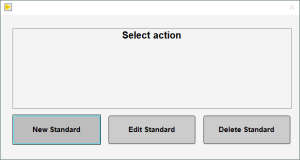
Figure 34. Action Prompt Window
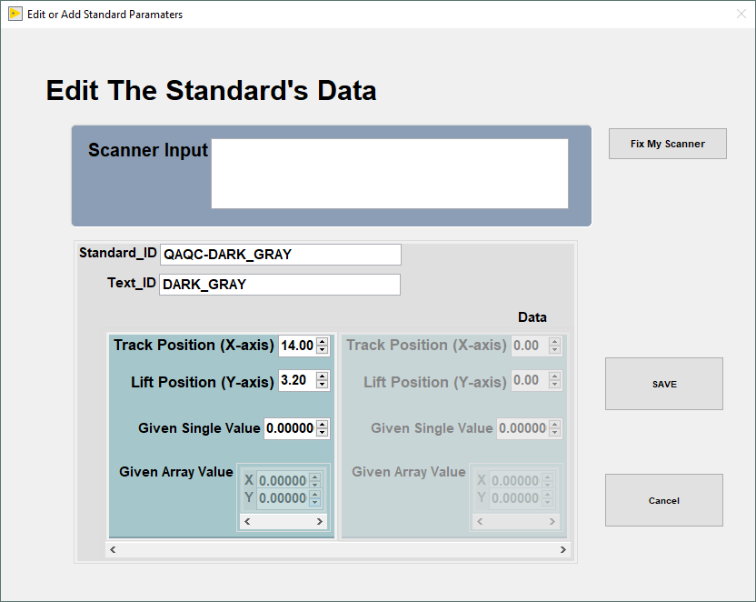
Figure 35. Edit Standard Window
QEPro: Lights ON
Select Instruments > QEPro: Lights ON. QEPro lights will turn ON.
QEPro: Lights OFF
Select Instruments > QEPro: Lights OFF. QEPro lights will turn OFF.
Y-Axis Setup
Select DAQ > Y-Axis Setup (Figure 3). The Y-axis LIFT Setup window will open (Figure 36). The Y-Axis setup is used to define the working distance for the AR700 laser. If anything is changed on the Y-axis mount, y-axis lift setup values should be determined experimentally.
- To determine the distance to benchmark, click the "Get Benchmark Data" button. This value is normally between 45.45 mm.
- The Touch Down Offset value is 4.00 cm.
- The Safe Clearance value (usually set to 3.0 cm) is used to prevent the sensors from running into something (e.g., a tall rock piece) that is higher than the section half liner.
- The Touch Compression value (usually set to 0.5 cm) is used to push downward gently after the landing to flatten the sensors against the core section.
Note: For very soft sediments, it may be necessary to set the Touch Compression to 0.0 cm.
The four Move to Buttons on the right are used to positioning the sensors in relation with the standards and with the initial point of the track. Use Motion Widget (select the Open MOTION Widget box) to set the sensors in the correct position. Then click Set. New values will be saved.
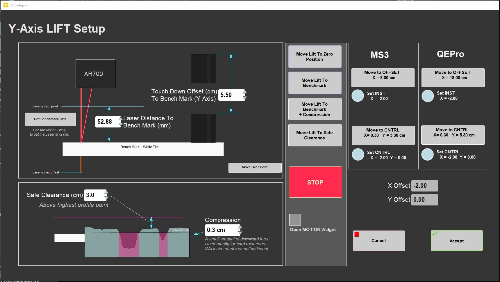
Figure 36. Y-Axis Utility window.
Measure Empty Liner
NOTE: This Utility should be manage by an technician. When these data are setup, only is necessary to perform another measurement a problem in the data was noticed or if the scientists are interested in obtaining a new profile.
Select DAQ >Measure Empty Liner (Figure 3). A window will pop up (Figure 37), prompting the user to start (MEASURE) or CANCEL the measurement. When clicking MEASURE the measurement will start immediately.
The empty core liner data will be substracted from the raw profile data to obtain the correct high of the core.
![]()
Figure 37. Empty liner measurement window.
Important: Use and empty liner with no end caps and as strait as possible to perform this experiment.
III. Uploading Data to LIMS
A. Data Upload Procedure
To upload the images into the database (LIMS) MegaUploadaTron (MUT) program must be running in background.
If not already started do the following:
- On the desktop click the MUT icon on the bottom task bar (Figure 39) and login with ship credentials. The LIMS Uploader window will appear (Figure 16).
- Once activated, the list of files from the C:\DATA\IN directory is displayed. Files are marked ready for upload by a green check mark.

Figure 38. MUT icon
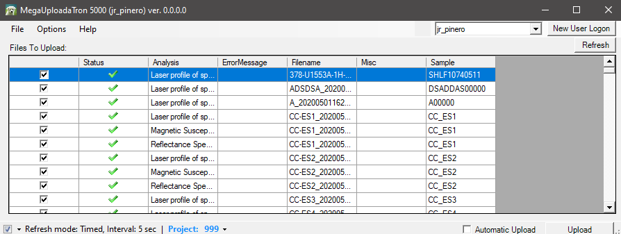
Figure 39. LIMS Uploader window
3. To manually upload files, check each file individually and clip upload. To automatically upload files, click on the Automatic Upload checkbox. The window can be minimized and MUT will be running in the background.
4. If files are marked by a purple question mark or red and white X icons, please contact a technician.
Purple question mark: Cannot identify the file.
Red and white X icons: Contains file errors.
5. Upon upload, data is moved to C:\DATA\Archive. If upload is unsuccessful, data is automatically moved to C:\DATA\Error. Please contact the PP technician is this occurs.
Data File Formats
Data upload files are text files used by the MUT application to load acquired data into LIMS. Files with the .RSC extension contain the reflectance spectroscopy and colorimetry data and files with the .MSPOINT extension contain the MS point data for a section. The files with a name containing PROFILE.csv are laser profiles for a given section.
The data upload files generated by the SHMSL are:
- .RSC: A data file containing all of the RSC measurements for a section of core. Data include: offset, L*, a*, b*, hue, chroma, x, y and z tristimulus, and sample time
- .MSPOINT: A data file containing all of the magnetic susceptibility point measurements for a section of core. Data include offset, magnetic susceptibility, and a time stamp. The file also includes the range and units and serial number of the magnetic susceptibility meter used.
- .PROFILE: a .file containing the section half ID and the observed core length measurement (cm).
Auxiliary Files
Auxiliary files are .csv formatted text files written for the AR700 laser, the QE Pro, and the MS point sensor. Each of these files is referenced in their respective upload file between the <File> tags and are archived in the ASMAN database.
The auxiliary files generated by the SHMSL are:
- rsc.csv: a summary file containing offset (cm), sensor temperature, dark pixel count, bin interval, the wavelength range measured, the integration time in microseconds, and the raw data values in each bin.
- mspoint.csv: a summary .csv file containing the mean magnetic susceptibility values for each measurement along a section as well as the range and units used at the time of measurement
- profile.csv: a summary .csv file containing the raw AR700 laser data for a section of core at 0.1mm steps. Data include offset, uncorrected height (mm), x-sect area (square mm), and benchmark (square cm).
Reflectance Spectroscopy and Colorimetry Files
- i_pi_gra.ini: A file containing the configuration information related to the GRA setup at the time of the measurement
- .RSC: A data file containing all of the RSC measurements for a section of core. Data include: offset, L*, a*, b*, hue, chroma, x, y and z tristimulus, and sample time
- rsc.csv: a summary file containing offset (cm), sensor temperature, dark pixel count, bin interval, the wavelength range measured, the integration time in microseconds, and the raw data values in each bin.
Magnetic Susceptibility Files
- i_pi_ms.ini: A file containing the configuration information related to the MS point sensor at the time of the measurement.
- .MSPOINT: A data file containing all of the magnetic susceptibility point measurements for a section of core. Data include offset, magnetic susceptibility, and a time stamp. The file also includes the range and units and serial number of the magnetic susceptibility meter used.
- mspoint.csv: a summary .csv file containing the mean magnetic susceptibility values for each measurement along a section as well as the range and units used at the time of measurement
AR700 Laser Profile Files
- i_pi_ar700.ini: A file containing the configuration information related to the AR700 displacement laser at the time of the given measurement
- .PROFILE: a .file containing the section half ID and the observed core length measurement (cm).
- profile.csv: a summary .csv file containing the raw AR700 laser data for a section of core at 0.1mm steps. Data include offset, uncorrected height (mm), x-sect area (square mm), and benchmark (square cm).
B. View and Verify Data
Data Available in LIVE
The data measured on each instrument can be viewed in real time on the LIMS information viewer (LIVE).
Choose the appropriate template (Ex: PHYS_PROPS_Summary), Expedition, Site, Hole or the needed restrictions and click View Data. The requested data will be displayed. You can travel in them by clicking on each of each core or section, which will enlarge the image.
Data Available in LORE
Each data set from the Section Half Multisensor Logger (SHMSL) is written to a file by section. The data for the RSC, MS-Point, and AR700 laser are each displayed under a different report in LORE. These reports are found under the Physical Properties heading and include Magnetic Susceptibility Point or Contact System (MSP) expanded report, Reflectance Spectroscopy and Colorimetry (RSC) expanded RSC, Reflectance Spectroscopy and Colorimetry (RSC) expanded PROFILE. The expanded reports include the linked original data files and more detailed information regarding the measurement.
Reflectance Spectroscopy and Colorimetry Standard Report
- Exp: Expedition number
- Site: Site number
- Hole: Hole number
- Core: Core number
- Type: Type indicates the coring tool used to recover the core (typical types are F, H, R, X).
- Sect: Section number
- A/W: Archive (A) or working (W) section half.
- Offset (cm): Position of the observation made, measured relative to the top of a section or section half.
- Depth CSF-A (m): Location of the observation expressed relative to the top of a hole.
- Depth [other] (m): Location of the observation expressed relative to the top of a hole. The location is presented in a scale selected by the science party or the report user.
- Reflectance L*: Lightness of the sample expressed in the CIELAB color space.
- Reflectance a*: Position of the color on the axis between red/magenta and green (negative = greater green character) in the CIELAB color space.
- Reflectance b*: Position of the color on the axis between yellow and blue (negative = greater blue character) in the CIELAB color space.
- Tristimulus X: X-component of the tristimulus value.
- Tristimulus Y: Y-component of the tristimulus value.
- Tristimulus Z: Z-component of the tristimulus value.
- Normalized spectral data: ASCII file with normalized spectral data.
- Unnormalized spectral data: ASCII file with unnormalized spectral data.
- Timestamp (UTC): Point in time at which the observation or set of observations was made.
- Instrument: An abbreviation or mnemonic for the spectrophotometric sensing device used to make this observation (OOUSB4000V).
- Instrument group: Abbreviation or mnemonic for the data collection device (logger) used to acquire this observation (SHMSL).
- Text ID: Automatically generated unique database identifier for a sample, visible on printed labels.
- Test No: Unique number associated with the instrument measurement steps that produced these data.
- Comments: Observer's notes about a measurement, the sample, or the measurement process.
Magnetic Susceptibility Point Standard Report
- Exp: Expedition number
- Site: Site number
- Hole: Hole number
- Core: Core number
- Type: Type indicates the coring tool used to recover the core (typical types are F, H, R, X).
- Sect: Section number
- A/W: Archive (A) or working (W) section half.
- Offset (cm): Position of the observation made, measured relative to the top of a section or section half.
- Depth CSF-A (m): Location of the observation expressed relative to the top of a hole.
- Depth [other] (m): Location of the observation expressed relative to the top of a hole. The location is presented in a scale selected by the science party or the report user.
- Magnetic susceptibility (SI): Magnetic susceptibility of the sample, volume-corrected as follows:
- MS2E sensor: magnetic susceptibility is reported in calibrated SI values, assuming the sample is a flat surface and has a depth greater than 10 mm
- MS2F sensor: magnetic susceptibility is reported in instrument units, converted to SI values by a geometric factor of 2 with the sensor placed against a flat surface
- MS2K sensor: magnetic susceptibility is reported in calibrated SI values, assuming the sample is a flat surface and has a depth greater than 10 mm
- Timestamp (UTC): Point in time at which an observation or set of observations was made on the logger.
- Instrument: An abbreviation or mnemonic for the sensing device used to make this observation.
- Instrument group: Abbreviation or mnemonic for the data collection device (logger) used to acquire this observation (SHMSL).
- Text ID: Automatically generated unique database identifier for a sample, visible on printed labels.
- Test No: Unique number associated with the instrument measurement steps that produced these data.
- Comments: Observer's notes about a measurement, the sample, or the measurement process.
C. Retrieve Data from LIMS
Expedition data can be downloaded from the database using the instrument Expanded Report on Download LIMS core data (LORE).
IV. Important Notes
Standards
Color Reflectance
- Labsphere, Inc. Spectralon® white standard, certified at 99% reflectivity (Figure 40).
- Labsphere, Inc. diffuse color reflectance targets:
- Grayscale: 99%, 50%, 20%, 2% reflectance (Referred to as white, light grey, dark grey, and black)
- Color: Red, Orange, Yellow, Green, Cyan, Blue, Purple, Violet (Figure 41).
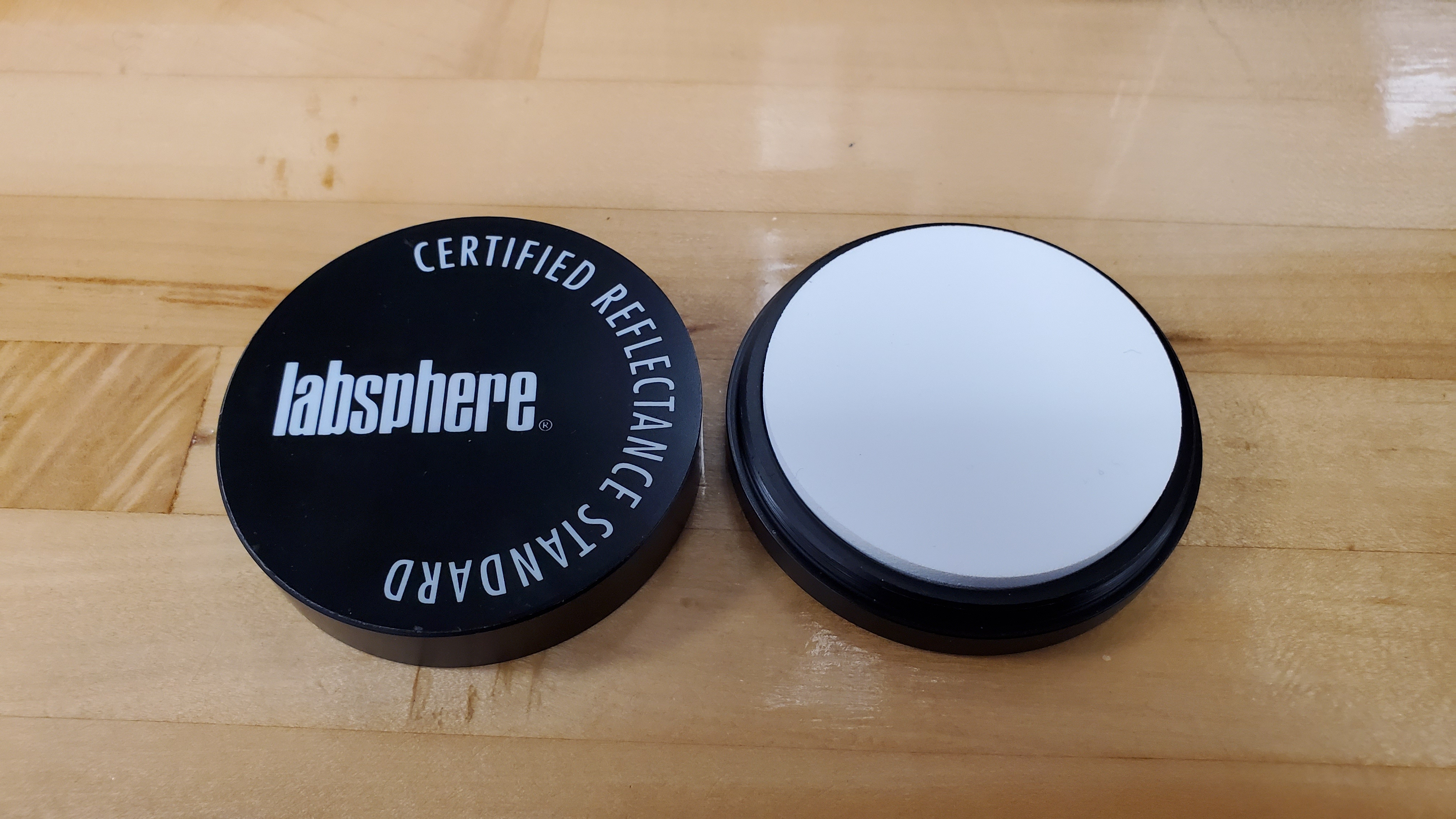 Figure 40. WHITE Spectralon® Calibration Standard
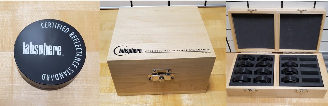
Figure 41. Spectralon Diffuse Standards.
Magnetic Susceptibility
The MS standards are used to check for drift, not to calibrate the meter or sensor. The JRSO puck is used to check drift instead of the Bartington standard because it is less sensitive to centering the sensor.
- Bartington-issued MS puck (note: user must center this standard carefully to get the correct reading)
- JRSO-created verification puck (~48 SIx10-6; mounted on track). The JRSO standard is made of Magnesium Oxide powder sealed inside a Petri dish with epoxy. The powder can be found in a PVC tube in the "MS Standards" drawer under the X-Ray track.
Data Handling–WORK IN PROGRESS
C:\data\IN
- Section half L* a* b* and XYZ data
- MS2K check standard result
- MS2K (MSPOINT) data file
- QE Pro white check standard result
- Laser profile file
C:\AUX_DATA\PROFILE
Laser profile data in 0.1 mm steps
C:\AUX_DATA\RSC\CALIB
White and Dark calibration spectral data per wavelength (380–900 in 2 nm steps)
C:\AUX_DATA\RSC\CNTRL
Raw spectra and normalized (% color reflectance) spectral data per wavelength (380–900 in 2 nm steps) for the white check standard at the end of a run
C:\AUX_DATA\RSC\RUN
Raw spectra and normalized (% color reflectance) spectral data per wavelength (380–900 in 2 nm steps) for the measured section.
Notes IMS v.12
- If 'Missing top' is selected the missing top will not be to reflected on the laser profile graph, but it will be on the MS and RSC graphs.
- Before using Motion Widget or Motion Utility to move the X-Axis, be sure that the sensors are set with safety distance from the core.
V. Appendix
A.1 Health, Safety & Environment
Safety
- Keep extraneous items and body parts away from the moving platform, belt, and motor.
- The track system has a well-marked emergency stop button to halt the system if needed.
- Do not look directly into the spectrometer light source.
- Do not look directly into the laser light source.
- Do not attempt to work on the system while a measurement is in progress.
- Do not lean over or onto the track.
- Do not stack anything on the track.
- This analytical system does not require personal protective equipment.
Pollution Prevention
This procedure does not generate heat or gases and requires no containment equipment.
Waste Management
Dispose of soiled GLAD® Plastic Wrap in an approved waste container.
A.2 Maintenance and Troubleshooting
Common Issues
Problem | Possible Causes | Solution |
MS sensor: baseline drift | Temperature variations | Ensure operating temperature is constant and preferably cool |
Make sure samples have equilibrated to room temperature | ||
MS sensor: systematic offset from MS2C data | MS2K/MS2E zeroing environment not the same as that for the samples | Check that the zeroing height is roughly equivalent to the height of a sample, and that no large metal objects have been introduced to the area |
MS sensor: reading fluctuations greater than ±1 least significant digit | External electrical noise | Check the operation area for: - large ferrous objects - heavy electrical machinery - radio frequency source devices |
Track is “stuck” | Gantry flag has tripped the end-of-travel limit switch | Adjust gantry flag and run sample again |
Current limit on motors was exceeded | Check the motor for LED error indicators. Call PP tech or ET to reset motor controller | |
Torque limit on motors was exceeded. | Call PP tech or ET to reset motor controller | |
Power supply voltage too low | Call PP tech or ET to check power supply input voltage | |
RSC values nonsensical/too bright | Ambient light level too high | Reduce ambient light level/ensure integration sphere makes flat contact with sample |
Laser sensor: no laser light/no laser range data | Configuration data lost | Press function button to restore factory default configuration |
Calibration data lost | Contact manufacturer | |
Laser sensor: LED flashes continuously at 1 Hz | Laser configuration incorrect | Call PP tech or ET to reset laser sensor |
Scheduled Maintenance
Daily
- Keep contact sensors and laser window clean by wiping with a Kimwipe.
- If necessary, use isopropyl alcohol to remove soil from sensors and laser window.
- Do not use any other solvent!
Annually
- Remove the end covers on the linear actuators and check if the motor belts need tightening.
- Examine the cable management system for abraded cables or other indications of wear.
- Remove the top covers of the linear actuators and check the ball screws to see if they need cleaning or additional lubrication.
When Needed
- If the reflectance standard becomes nicked or soiled, it can be smoothed, flattened, and cleaned.
B.1 IMS Program Structure
a) IMS Program Structure
IMS is a modular program. Individual modules are as follows:
- Config Files: Unique for each track. Used for initialize the track and set up default parameters.
- Documents: Important Information related with configuration setup.
- Error: IMS error file.
- FRIENDS: Systems that use IMS but don't use DAQ Engine.
- IMS Common: Programs that are used by different instruments.
- PLUG-INS: Code for each of the instruments.
- Projects: Main IMS libraries.
- Resources: Other information and programs needed to run IMS.
- UI: User Interface
- X-CONFIG: .ini files, specifics for each instrument.
- MOTION plug-in: Codes for the motion control system.
- DAQ Engine: Code that organizes INST and MOTION plug-ins into a track system.
The IMS Main User Interface (UI) calls these modules, instructs them to initialize, and provides a user interface to their functionality.
The SHMSL system, specifically, is built with three INST modules (MS3, QEPro, AR700), two MOTION modules (X-axis, Y-axis), and one DAQ Engine module.
The IMS Main User Interface (UI) calls these modules, instructs them to initialize, and provides a user interface to their functionality.
Each module manages a configuration file that opens the IMS program at the same state it was when previously closed and provides utilities for the user to edit or modify the configuration data and calibration routines.
b) Communication and Control Setup
Data communication and control is USB based and managed via National Instrument’s Measurement & Automation Explorer (NI-MAX). When you open NI-MAX and expand the Device and Interface section. The correct communications setup can be found at IMS Hardware Communications Setup.
B.2 Motion Control Setup
Select Motion > Setup from the main IMS-SHMSL window (Figure 3).
Motion control should be set during initial setup and further changes should not be necessary. The M-Drive Motion Setup control panel will open (Figure 42).
- The user may select between four setup panels from this window.
- Motor and Track Options
- Fixed Positions
- Limit and Home Switches
- Motion Profiles

Figure 42. Motion Setup Menu
Motor and Track Options menu
Once these values have been properly set, they should not change. This panel is only for initial setup.
- Make sure to use the values shown for the SHMSL (Figure 43).
The relationship between motor revolutions and linear motion of the track is defined in this window and is critical to both safe and accurate operation. User should be familiar with the M-Drive motor system prior to adjusting these settings. These values are used by IMS to set motion controller parameters and convert encoder pulses into ± position values in centimeters. The correct settings for the SHMSL are as follows:
X-Axis Track Motor Setup Settings
- Encoder Pulses/rev: 2048
- Screw Pitch: 2.00000E+0
- Gear Ratio: 4.00000
- Direction of Positive Motion: CCW for positive encoder counts
Y-Axis Track Motor Setup Settings
- Encoder Pulses/rev: 2048
- Screw Pitch: 1.00000E+0
- Gear Ratio: 1.00000
- Direction of Positive Motion: CW for positive encoder counts.
Click the Motion Utlity button to open the Motion Utility window (Figure 44) and test the settings. Click Close to exit this window.
Click Accept to save the values or Cancel to return to previous values.

Figure 43. Track Motor Setup for the X-axis motor (left) and the Y-axis motor (right).

Figure 44. Motion Utility Window
Fixed Positions menu
Once these values have been properly set, they should not change. This panel is only for initial setup.
In this window the user may define fixed track locations used by IMS motion control. For the SHMSL make sure to use these value unless there has been a physical change to the system (Figure 45).
X-Axis Fixed Position Settings
- Max Section Length: 160.0 cm
- Track Length: 200.0 cm
- Load Position: -4.0 cm
- Unload Position: 170.0 cm
- All "PUSH Track Only" settings = OFF (or 0.0, as appropriate)
Y-Axis Fixed Position Settings
- Max Section Length: not configurable for this axis
- Track Length: not configurable for this axis
- Load Position: -3.0 cm
- Unload Position: -3.0 cm
- All "PUSH Track Only" settings = OFF.
Click the Motion Utiilty button to open the Motion Utility window (Figure 44) and test the settings. Click Close to exit this window.
Click Done to save the settings. Click Cancel to return to previous values.
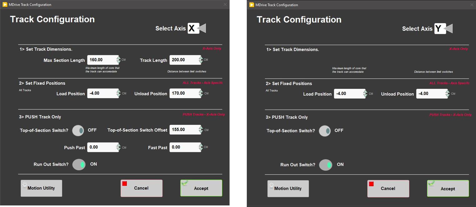
Figure 45. Track Configuration values for the X-axis (left) and Y-axis (right).
Track Configure – Limit & Home Switches
Once these values have been properly set, they should not change. This panel is only for initial setup.
The SHMSL X-axis (down-core motion) and Y-axis (vertical sensor motion) are configured using this screen (Figure 46). The X-axis is "CW Look @ CCW Edge" logic. The Y-axis is "CCW Look @ CCW Edge" logic.
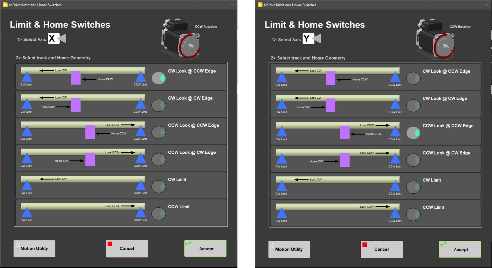
Figure 46. X-Axis (left) and Y-Axis (right) Limit and Home Switch Configuration
Motion Profile
The motion profiles window can be used to adjust the speed and acceleration profiles used by the track for various types of movements (Figure 47).
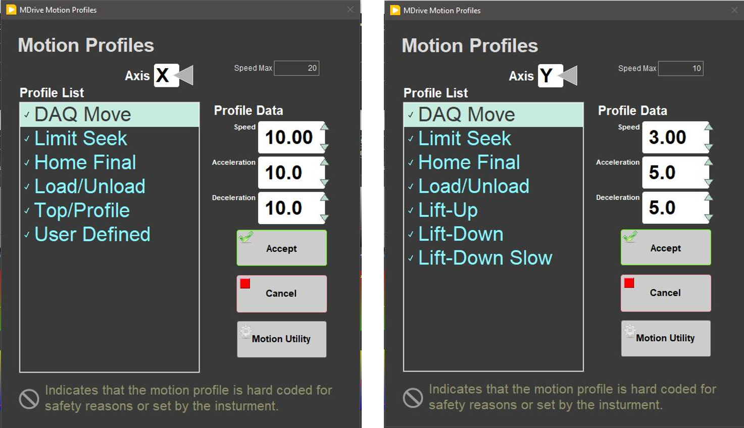
Figure 47. X-Axis (left) and Y-Axis (right) Motion Profiles
The following table shows the motion profile settings for the SHMSL X and Y axes controlled by the interface.
Axis→ | X-Axis | Y-Axis | ||||
|---|---|---|---|---|---|---|
Profile↓ | Speed | Accel. | Decel. | Speed | Accel. | Decel. |
DAQ Move | 10.0 | 10.0 | 10.00 | 3.0 | 5.0 | 5.0 |
Limit Seek | 2.0 | 5.0 | 30.0 | 3.0 | 10.0 | 80.0 |
Home Final | 1.0 | 3.0 | 20.0 | 1.0 | 10.0 | 80.0 |
Load/Unload | 25.0 | 5.0 | 10.0 | 10.0 | 5.0 | 5.0 |
Top/Profile | 5.0 | 20.0 | 10.0 | N/A | N/A | N/A |
User Defined | 20.0 | 5.0 | 5.0 | N/A | N/A | N/A |
Lift-Up | N/A | N/A | N/A | 5.0 | 5.0 | 5.0 |
Lift-Down | N/A | N/A | N/A | 5.0 | 5.0 | 5.0 |
Lift-Down Slow | N/A | N/A | N/A | 3.0 | 5.0 | 5.0 |
Table: Motion Profile by Axis for SHMSL
NOTE: These parameters are set for make the measurement efficient (quality-time). It is always possible to set them lower to increase the quality when cores are more irregular. Ex: Lower the speed of the Top/Profile to 2.00 or 3.00.
B.3 LIMS Component Tables
The following LIMS component tables are included here:
- MSPOINT - magnetic susceptibility by contact/point sensor measurements
- PROFILE - laser profile of the surface of the core section
- RSC - color reflectance measurements
| ANALYSIS | TABLE | NAME | ABOUT TEXT |
| MSPOINT | SAMPLE | Exp | Exp: expedition number |
| MSPOINT | SAMPLE | Site | Site: site number |
| MSPOINT | SAMPLE | Hole | Hole: hole number |
| MSPOINT | SAMPLE | Core | Core: core number |
| MSPOINT | SAMPLE | Type | Type: type indicates the coring tool used to recover the core (typical types are F, H, R, X). |
| MSPOINT | SAMPLE | Sect | Sect: section number |
| MSPOINT | SAMPLE | A/W | A/W: archive (A) or working (W) section half. |
| MSPOINT | SAMPLE | text_id | Text_ID: automatically generated database identifier for a sample, also carried on the printed labels. This identifier is guaranteed to be unique across all samples. |
| MSPOINT | SAMPLE | sample_number | Sample Number: automatically generated database identifier for a sample. This is the primary key of the SAMPLE table. |
| MSPOINT | SAMPLE | label_id | Label identifier: automatically generated, human readable name for a sample that is printed on labels. This name is not guaranteed unique across all samples. |
| MSPOINT | SAMPLE | sample_name | Sample name: short name that may be specified for a sample. You can use an advanced filter to narrow your search by this parameter. |
| MSPOINT | SAMPLE | x_sample_state | Sample state: Single-character identifier always set to "W" for samples; standards can vary. |
| MSPOINT | SAMPLE | x_project | Project: similar in scope to the expedition number, the difference being that the project is the current cruise, whereas expedition could refer to material/results obtained on previous cruises |
| MSPOINT | SAMPLE | x_capt_loc | Captured location: "captured location," this field is usually null and is unnecessary because any sample captured on the JR has a sample_number ending in 1, and GCR ending in 2 |
| MSPOINT | SAMPLE | location | Location: location that sample was taken; this field is usually null and is unnecessary because any sample captured on the JR has a sample_number ending in 1, and GCR ending in 2 |
| MSPOINT | SAMPLE | x_sampling_tool | Sampling tool: sampling tool used to take the sample (e.g., syringe, spatula) |
| MSPOINT | SAMPLE | changed_by | Changed by: username of account used to make a change to a sample record |
| MSPOINT | SAMPLE | changed_on | Changed on: date/time stamp for change made to a sample record |
| MSPOINT | SAMPLE | sample_type | Sample type: type of sample from a predefined list (e.g., HOLE, CORE, LIQ) |
| MSPOINT | SAMPLE | x_offset | Offset (m): top offset of sample from top of parent sample, expressed in meters. |
| MSPOINT | SAMPLE | x_offset_cm | Offset (cm): top offset of sample from top of parent sample, expressed in centimeters. This is a calculated field (offset, converted to cm) |
| MSPOINT | SAMPLE | x_bottom_offset_cm | Bottom offset (cm): bottom offset of sample from top of parent sample, expressed in centimeters. This is a calculated field (offset + length, converted to cm) |
| MSPOINT | SAMPLE | x_diameter | Diameter (cm): diameter of sample, usually applied only to CORE, SECT, SHLF, and WRND samples; however this field is null on both Exp. 390 and 393, so it is no longer populated by Sample Master |
| MSPOINT | SAMPLE | x_orig_len | Original length (m): field for the original length of a sample; not always (or reliably) populated |
| MSPOINT | SAMPLE | x_length | Length (m): field for the length of a sample [as entered upon creation] |
| MSPOINT | SAMPLE | x_length_cm | Length (cm): field for the length of a sample. This is a calculated field (length, converted to cm). |
| MSPOINT | SAMPLE | status | Status: single-character code for the current status of a sample (e.g., active, canceled) |
| MSPOINT | SAMPLE | old_status | Old status: single-character code for the previous status of a sample; used by the LIME program to restore a canceled sample |
| MSPOINT | SAMPLE | original_sample | Original sample: field tying a sample below the CORE level to its parent HOLE sample |
| MSPOINT | SAMPLE | parent_sample | Parent sample: the sample from which this sample was taken (e.g., for PWDR samples, this might be a SHLF or possibly another PWDR) |
| MSPOINT | SAMPLE | standard | Standard: T/F field to differentiate between samples (standard=F) and QAQC standards (standard=T) |
| MSPOINT | SAMPLE | login_by | Login by: username of account used to create the sample (can be the LIMS itself [e.g., SHLFs created when a SECT is created]) |
| MSPOINT | SAMPLE | login_date | Login date: creation date of the sample |
| MSPOINT | SAMPLE | legacy | Legacy flag: T/F indicator for when a sample is from a previous expedition and is locked/uneditable on this expedition |
| MSPOINT | TEST | test changed_on | TEST changed on: date/time stamp for a change to a test record. |
| MSPOINT | TEST | test status | TEST status: single-character code for the current status of a test (e.g., active, in process, canceled) |
| MSPOINT | TEST | test old_status | TEST old status: single-character code for the previous status of a test; used by the LIME program to restore a canceled test |
| MSPOINT | TEST | test test_number | TEST test number: automatically generated database identifier for a test record. This is the primary key of the TEST table. |
| MSPOINT | TEST | test date_received | TEST date received: date/time stamp for the creation of the test record. |
| MSPOINT | TEST | test instrument | TEST instrument [instrument group]: field that describes the instrument group (most often this applies to loggers with multiple sensors); often obscure (e.g., user_input) |
| MSPOINT | TEST | test analysis | TEST analysis: analysis code associated with this test (foreign key to the ANALYSIS table) |
| MSPOINT | TEST | test x_project | TEST project: similar in scope to the expedition number, the difference being that the project is the current cruise, whereas expedition could refer to material/results obtained on previous cruises |
| MSPOINT | TEST | test sample_number | TEST sample number: the sample_number of the sample to which this test record is attached; a foreign key to the SAMPLE table |
| MSPOINT | CALCULATED | Depth CSF-A (m) | Depth CSF-A (m): position of observation expressed relative to the top of the hole. |
| MSPOINT | CALCULATED | Depth CSF-B (m) | Depth [other] (m): position of observation expressed relative to the top of the hole. The location is presented in a scale selected by the science party or the report user. |
| MSPOINT | RESULT | aux_file_asman_id | RESULT auxiliary file ASMAN_ID: serial number of the ASMAN link for the auxiliary data file |
| MSPOINT | RESULT | aux_file_filename | RESULT auxiliary filename: file name of the auxiliary data file |
| MSPOINT | RESULT | config_asman_id | RESULT config file ASMAN_ID: serial number of the ASMAN link for the configuration file |
| MSPOINT | RESULT | config_filename | RESULT config filename: file name of the configuration file |
| MSPOINT | RESULT | magnetic_susceptibility | RESULT magnetic susceptibility (SI x 10^-6): magnetic susceptibility is reported in calibrated SI values, assuming the sample is a flat surface and has a depth greater than 10 mm |
| MSPOINT | RESULT | ms_correction | RESULT probe correction factor: geometric correction factor for MS probe (2.0 for MS2F, 1.0 for MS2E or MS2K) |
| MSPOINT | RESULT | ms_sample_integration_time | RESULT integration time (ms): integration time for the MS3 measurement |
| MSPOINT | RESULT | ms_units | RESULT MS units: shows whether the meter was set to SI or cgs units |
| MSPOINT | RESULT | ms_zero | RESULT zero height (cm): height above the track the zeroing of the meter was performed |
| MSPOINT | RESULT | ms_zero_integration_time | RESULT zero integration time (ms): integration time for the meter zeroing action |
| MSPOINT | RESULT | observed_length (cm) | RESULT observed length (cm): the length of the section half as entered by the user |
| MSPOINT | RESULT | offset (cm) | RESULT offset (cm): position of the observation made, measured relative to the top of a section half. |
| MSPOINT | RESULT | run_asman_id | RESULT run file ASMAN_ID: serial number of the ASMAN link for the run (.MSPOINT) file |
| MSPOINT | RESULT | run_filename | RESULT run filename: file name for the run (.MSPOINT) file |
| MSPOINT | RESULT | time_since_zero | RESULT time since last zero (s): time since the last zeroing action |
| MSPOINT | RESULT | timestamp | RESULT timestamp: date/time stamp for each individual measurement |
| MSPOINT | RESULT | zero_timestamp | RESULT zeroing action timestamp: date/time stamp for the zeroing action |
| MSPOINT | SAMPLE | sample description | SAMPLE comment: contents of the SAMPLE.description field, usually shown on reports as "Sample comments" |
| MSPOINT | TEST | test test_comment | TEST comment: contents of the TEST.comment field, usually shown on reports as "Test comments" |
| MSPOINT | RESULT | result comments | RESULT comment: contents of a result parameter with name = "comment," usually shown on reports as "Result comments" |
| ANALYSIS | TABLE | NAME | ABOUT TEXT |
| PROFILE | SAMPLE | Exp | Exp: expedition number |
| PROFILE | SAMPLE | Site | Site: site number |
| PROFILE | SAMPLE | Hole | Hole: hole number |
| PROFILE | SAMPLE | Core | Core: core number |
| PROFILE | SAMPLE | Type | Type: type indicates the coring tool used to recover the core (typical types are F, H, R, X). |
| PROFILE | SAMPLE | Sect | Sect: section number |
| PROFILE | SAMPLE | A/W | A/W: archive (A) or working (W) section half. |
| PROFILE | SAMPLE | text_id | Text_ID: automatically generated database identifier for a sample, also carried on the printed labels. This identifier is guaranteed to be unique across all samples. |
| PROFILE | SAMPLE | sample_number | Sample Number: automatically generated database identifier for a sample. This is the primary key of the SAMPLE table. |
| PROFILE | SAMPLE | label_id | Label identifier: automatically generated, human readable name for a sample that is printed on labels. This name is not guaranteed unique across all samples. |
| PROFILE | SAMPLE | sample_name | Sample name: short name that may be specified for a sample. You can use an advanced filter to narrow your search by this parameter. |
| PROFILE | SAMPLE | x_sample_state | Sample state: Single-character identifier always set to "W" for samples; standards can vary. |
| PROFILE | SAMPLE | x_project | Project: similar in scope to the expedition number, the difference being that the project is the current cruise, whereas expedition could refer to material/results obtained on previous cruises |
| PROFILE | SAMPLE | x_capt_loc | Captured location: "captured location," this field is usually null and is unnecessary because any sample captured on the JR has a sample_number ending in 1, and GCR ending in 2 |
| PROFILE | SAMPLE | location | Location: location that sample was taken; this field is usually null and is unnecessary because any sample captured on the JR has a sample_number ending in 1, and GCR ending in 2 |
| PROFILE | SAMPLE | x_sampling_tool | Sampling tool: sampling tool used to take the sample (e.g., syringe, spatula) |
| PROFILE | SAMPLE | changed_by | Changed by: username of account used to make a change to a sample record |
| PROFILE | SAMPLE | changed_on | Changed on: date/time stamp for change made to a sample record |
| PROFILE | SAMPLE | sample_type | Sample type: type of sample from a predefined list (e.g., HOLE, CORE, LIQ) |
| PROFILE | SAMPLE | x_offset | Offset (m): top offset of sample from top of parent sample, expressed in meters. |
| PROFILE | SAMPLE | x_offset_cm | Offset (cm): top offset of sample from top of parent sample, expressed in centimeters. This is a calculated field (offset, converted to cm) |
| PROFILE | SAMPLE | x_bottom_offset_cm | Bottom offset (cm): bottom offset of sample from top of parent sample, expressed in centimeters. This is a calculated field (offset + length, converted to cm) |
| PROFILE | SAMPLE | x_diameter | Diameter (cm): diameter of sample, usually applied only to CORE, SECT, SHLF, and WRND samples; however this field is null on both Exp. 390 and 393, so it is no longer populated by Sample Master |
| PROFILE | SAMPLE | x_orig_len | Original length (m): field for the original length of a sample; not always (or reliably) populated |
| PROFILE | SAMPLE | x_length | Length (m): field for the length of a sample [as entered upon creation] |
| PROFILE | SAMPLE | x_length_cm | Length (cm): field for the length of a sample. This is a calculated field (length, converted to cm). |
| PROFILE | SAMPLE | status | Status: single-character code for the current status of a sample (e.g., active, canceled) |
| PROFILE | SAMPLE | old_status | Old status: single-character code for the previous status of a sample; used by the LIME program to restore a canceled sample |
| PROFILE | SAMPLE | original_sample | Original sample: field tying a sample below the CORE level to its parent HOLE sample |
| PROFILE | SAMPLE | parent_sample | Parent sample: the sample from which this sample was taken (e.g., for PWDR samples, this might be a SHLF or possibly another PWDR) |
| PROFILE | SAMPLE | standard | Standard: T/F field to differentiate between samples (standard=F) and QAQC standards (standard=T) |
| PROFILE | SAMPLE | login_by | Login by: username of account used to create the sample (can be the LIMS itself [e.g., SHLFs created when a SECT is created]) |
| PROFILE | SAMPLE | login_date | Login date: creation date of the sample |
| PROFILE | SAMPLE | legacy | Legacy flag: T/F indicator for when a sample is from a previous expedition and is locked/uneditable on this expedition |
| PROFILE | TEST | test changed_on | TEST changed on: date/time stamp for a change to a test record. |
| PROFILE | TEST | test status | TEST status: single-character code for the current status of a test (e.g., active, in process, canceled) |
| PROFILE | TEST | test old_status | TEST old status: single-character code for the previous status of a test; used by the LIME program to restore a canceled test |
| PROFILE | TEST | test test_number | TEST test number: automatically generated database identifier for a test record. This is the primary key of the TEST table. |
| PROFILE | TEST | test date_received | TEST date received: date/time stamp for the creation of the test record. |
| PROFILE | TEST | test instrument | TEST instrument [instrument group]: field that describes the instrument group (most often this applies to loggers with multiple sensors); often obscure (e.g., user_input) |
| PROFILE | TEST | test analysis | TEST analysis: analysis code associated with this test (foreign key to the ANALYSIS table) |
| PROFILE | TEST | test x_project | TEST project: similar in scope to the expedition number, the difference being that the project is the current cruise, whereas expedition could refer to material/results obtained on previous cruises |
| PROFILE | TEST | test sample_number | TEST sample number: the sample_number of the sample to which this test record is attached; a foreign key to the SAMPLE table |
| PROFILE | CALCULATED | Top depth CSF-A (m) | Top depth CSF-A (m): position of observation expressed relative to the top of the hole. |
| PROFILE | CALCULATED | Bottom depth CSF-A (m) | Bottom depth CSF-A (m): position of observation expressed relative to the top of the hole. |
| PROFILE | CALCULATED | Top depth CSF-B (m) | Top depth [other] (m): position of observation expressed relative to the top of the hole. The location is presented in a scale selected by the science party or the report user. |
| PROFILE | CALCULATED | Bottom depth CSF-B (m) | Bottom depth [other] (m): position of observation expressed relative to the top of the hole. The location is presented in a scale selected by the science party or the report user. |
| PROFILE | RESULT | config_asman_id | RESULT config file ASMAN_ID: serial number of the ASMAN link for the configuration file |
| PROFILE | RESULT | config_filename | RESULT config filename: file name of the configuration file |
| PROFILE | RESULT | observed_length (cm) | RESULT observed length (cm): length of the section as recorded by the core logger track |
| PROFILE | RESULT | profile_asman_id | RESULT laser profile data ASMAN_ID: serial number of the ASMAN link for the laser profile raw data file (0.01 cm resolution) |
| PROFILE | RESULT | profile_filename | RESULT laser profile data filename: file name of the laser profile raw data file (0.01 cm resolution) |
| PROFILE | RESULT | run_asman_id | RESULT run ASMAN_ID: serial number of the ASMAN link for the run (.GRA) file |
| PROFILE | RESULT | run_filename | RESULT run filename: file name of the run (.GRA) file |
| PROFILE | SAMPLE | sample description | SAMPLE comment: contents of the SAMPLE.description field, usually shown on reports as "Sample comments" |
| PROFILE | TEST | test test_comment | TEST comment: contents of the TEST.comment field, usually shown on reports as "Test comments" |
| PROFILE | RESULT | result comments | RESULT comment: contents of a result parameter with name = "comment," usually shown on reports as "Result comments" |
| ANALYSIS | TABLE | NAME | ABOUT TEXT |
| RSC | SAMPLE | Exp | Exp: expedition number |
| RSC | SAMPLE | Site | Site: site number |
| RSC | SAMPLE | Hole | Hole: hole number |
| RSC | SAMPLE | Core | Core: core number |
| RSC | SAMPLE | Type | Type: type indicates the coring tool used to recover the core (typical types are F, H, R, X). |
| RSC | SAMPLE | Sect | Sect: section number |
| RSC | SAMPLE | A/W | A/W: archive (A) or working (W) section half. |
| RSC | SAMPLE | text_id | Text_ID: automatically generated database identifier for a sample, also carried on the printed labels. This identifier is guaranteed to be unique across all samples. |
| RSC | SAMPLE | sample_number | Sample Number: automatically generated database identifier for a sample. This is the primary key of the SAMPLE table. |
| RSC | SAMPLE | label_id | Label identifier: automatically generated, human readable name for a sample that is printed on labels. This name is not guaranteed unique across all samples. |
| RSC | SAMPLE | sample_name | Sample name: short name that may be specified for a sample. You can use an advanced filter to narrow your search by this parameter. |
| RSC | SAMPLE | x_sample_state | Sample state: Single-character identifier always set to "W" for samples; standards can vary. |
| RSC | SAMPLE | x_project | Project: similar in scope to the expedition number, the difference being that the project is the current cruise, whereas expedition could refer to material/results obtained on previous cruises |
| RSC | SAMPLE | x_capt_loc | Captured location: "captured location," this field is usually null and is unnecessary because any sample captured on the JR has a sample_number ending in 1, and GCR ending in 2 |
| RSC | SAMPLE | location | Location: location that sample was taken; this field is usually null and is unnecessary because any sample captured on the JR has a sample_number ending in 1, and GCR ending in 2 |
| RSC | SAMPLE | x_sampling_tool | Sampling tool: sampling tool used to take the sample (e.g., syringe, spatula) |
| RSC | SAMPLE | changed_by | Changed by: username of account used to make a change to a sample record |
| RSC | SAMPLE | changed_on | Changed on: date/time stamp for change made to a sample record |
| RSC | SAMPLE | sample_type | Sample type: type of sample from a predefined list (e.g., HOLE, CORE, LIQ) |
| RSC | SAMPLE | x_offset | Offset (m): top offset of sample from top of parent sample, expressed in meters. |
| RSC | SAMPLE | x_offset_cm | Offset (cm): top offset of sample from top of parent sample, expressed in centimeters. This is a calculated field (offset, converted to cm) |
| RSC | SAMPLE | x_bottom_offset_cm | Bottom offset (cm): bottom offset of sample from top of parent sample, expressed in centimeters. This is a calculated field (offset + length, converted to cm) |
| RSC | SAMPLE | x_diameter | Diameter (cm): diameter of sample, usually applied only to CORE, SECT, SHLF, and WRND samples; however this field is null on both Exp. 390 and 393, so it is no longer populated by Sample Master |
| RSC | SAMPLE | x_orig_len | Original length (m): field for the original length of a sample; not always (or reliably) populated |
| RSC | SAMPLE | x_length | Length (m): field for the length of a sample [as entered upon creation] |
| RSC | SAMPLE | x_length_cm | Length (cm): field for the length of a sample. This is a calculated field (length, converted to cm). |
| RSC | SAMPLE | status | Status: single-character code for the current status of a sample (e.g., active, canceled) |
| RSC | SAMPLE | old_status | Old status: single-character code for the previous status of a sample; used by the LIME program to restore a canceled sample |
| RSC | SAMPLE | original_sample | Original sample: field tying a sample below the CORE level to its parent HOLE sample |
| RSC | SAMPLE | parent_sample | Parent sample: the sample from which this sample was taken (e.g., for PWDR samples, this might be a SHLF or possibly another PWDR) |
| RSC | SAMPLE | standard | Standard: T/F field to differentiate between samples (standard=F) and QAQC standards (standard=T) |
| RSC | SAMPLE | login_by | Login by: username of account used to create the sample (can be the LIMS itself [e.g., SHLFs created when a SECT is created]) |
| RSC | SAMPLE | login_date | Login date: creation date of the sample |
| RSC | SAMPLE | legacy | Legacy flag: T/F indicator for when a sample is from a previous expedition and is locked/uneditable on this expedition |
| RSC | TEST | test changed_on | TEST changed on: date/time stamp for a change to a test record. |
| RSC | TEST | test status | TEST status: single-character code for the current status of a test (e.g., active, in process, canceled) |
| RSC | TEST | test old_status | TEST old status: single-character code for the previous status of a test; used by the LIME program to restore a canceled test |
| RSC | TEST | test test_number | TEST test number: automatically generated database identifier for a test record. This is the primary key of the TEST table. |
| RSC | TEST | test date_received | TEST date received: date/time stamp for the creation of the test record. |
| RSC | TEST | test instrument | TEST instrument [instrument group]: field that describes the instrument group (most often this applies to loggers with multiple sensors); often obscure (e.g., user_input) |
| RSC | TEST | test analysis | TEST analysis: analysis code associated with this test (foreign key to the ANALYSIS table) |
| RSC | TEST | test x_project | TEST project: similar in scope to the expedition number, the difference being that the project is the current cruise, whereas expedition could refer to material/results obtained on previous cruises |
| RSC | TEST | test sample_number | TEST sample number: the sample_number of the sample to which this test record is attached; a foreign key to the SAMPLE table |
| RSC | CALCULATED | Depth CSF-A (m) | Depth CSF-A (m): position of observation expressed relative to the top of the hole. |
| RSC | CALCULATED | Depth CSF-B (m) | Depth [other] (m): position of observation expressed relative to the top of the hole. The location is presented in a scale selected by the science party or the report user. |
| RSC | RESULT | calibration_valid | RESULT calibration valid: a field to indicate whether the calibration was inside its expiration time when the measurement was made |
| RSC | RESULT | chroma | RESULT chroma: colorfulness of the sample judged as a propotion of the brightness of the white target |
| RSC | RESULT | cielab_a_star | RESULT CIELAB a*: position of the color on the axis between red/magenta and green (negative = greater green character) in the CIELAB color space. |
| RSC | RESULT | cielab_b_star | RESULT CIELAB b*: position of the color on the axis between yellow and blue (negative = greater blue character) in the CIELAB color space. |
| RSC | RESULT | cielab_l_star | RESULT CIELAB L*: lightness of the sample expressed in the CIELAB color space. |
| RSC | RESULT | config_asman_id | RESULT config file ASMAN_ID: serial number of the ASMAN link for the configuration file |
| RSC | RESULT | config_filename | RESULT config filename: file name of the configuration file |
| RSC | RESULT | geometry | RESULT geometry: the geometry for the sensor, sample, and illuminant (in our case, d/8, specular component excluded, which means lighting comes in from 8 degrees from vertical and the sensor is perpendicular to the integration sphere wall |
| RSC | RESULT | hue | RESULT hue: the degree to which a stimulus can be described as similar to or different from stimuli that are described as red, orange, yellow, green, blue, violet |
| RSC | RESULT | illuminant | RESULT illuminant: the theoretical source of visible light with a given spectral power (e.g., 5000 K for D50; we use D50) |
| RSC | RESULT | observed_length (cm) | RESULT observed length (cm): length of the section as recorded by the core logger track |
| RSC | RESULT | observer | RESULT observer: tristimulus (and other color space) values depend on the observer's field of view; the standard observer is a 2 degree arc inside the fovea; IODP uses both 10 degree and 2 degree |
| RSC | RESULT | offset (cm) | RESULT offset (cm): position of the observation made, measured relative to the top of a section half. |
| RSC | RESULT | rsc_norm_asman_id | RESULT normalized color reflectance ASMAN_ID: serial number of the ASMAN link for the normalized (% reflectance) spectral file |
| RSC | RESULT | rsc_norm_filename | RESULT normalized color reflectance filename: file name of the normalized (% reflectance) spectral file |
| RSC | RESULT | rsc_raw_asman_id | RESULT raw color reflectance ASMAN_ID: serial number of the ASMAN link for the raw (reflected intensity) spectral file |
| RSC | RESULT | rsc_raw_filename | RESULT raw color reflectance filename: file name of the raw (reflected intensity) spectral file |
| RSC | RESULT | run_asman_id | RESULT run file ASMAN_ID: serial number of the ASMAN link for the run (.RSC) file |
| RSC | RESULT | run_filename | RESULT run filename: file name of the run (.RSC) file |
| RSC | RESULT | sample_time (ns) | RESULT sample integration time (ns): Time for the measurement on samples |
| RSC | RESULT | standard_time (ns) | RESULT standard integration time (ns): Time for the measurement on standards (only populated during QC check or calibration) |
| RSC | RESULT | timestamp | RESULT timestamp: Time/date stamp for each individual measurement |
| RSC | RESULT | tristimulus_x | RESULT Tristimulus X value: CIELAB Tristimulus X component of the color space |
| RSC | RESULT | tristimulus_y | RESULT Tristimulus Y value: CIELAB Tristimulus Y component of the color space |
| RSC | RESULT | tristimulus_z | RESULT Tristimulus Z value: CIELAB Tristimulus Z component of the color space |
| RSC | RESULT | value | RESULT value: lightness value in the HSV representation of the RGB color model |
| RSC | SAMPLE | sample description | SAMPLE comment: contents of the SAMPLE.description field, usually shown on reports as "Sample comments" |
| RSC | TEST | test test_comment | TEST comment: contents of the TEST.comment field, usually shown on reports as "Test comments" |
| RSC | RESULT | result comments | RESULT comment: contents of a result parameter with name = "comment," usually shown on reports as "Result comments" |
C.1 Hardware
The SHMSL system consists of the following hardware components (Figure 48):
- Bartington MS2K or MS2E (Note: MS2E is not generally recommended because of its very small read area) magnetic susceptibility contact probe
- Bartington MS2 meter, run in serial communications mode
- Ocean Optics QE Pro visible spectrum spectrophotometer
- Ocean Optics HL-2000 Halogen Light Source with Attenuator and TTL-Shutter
- Ocean Optics Multi-LED BluLoop Light Source
- Ocean Optics 30 mm integrating sphere, with a 10 mm aperture
- Acuity AccuRange AR700 Laser
- Barcode scanner
- Instrument platform
- Hardware abort switch
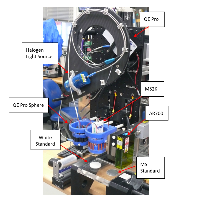
Figure 48. SHMSL Hardware
Bartington MS2K Probe Susceptibility Contact Probe
Specification | Value |
Dimensions (mm) | 165 x 145 x 50mm |
Operating frequency (kHz) | 0.930 |
Depth of Response | 50% at 3mm |
Measurement period: |
|
Temperature induced drift | <2 x 10⁻⁵ SI in 5 min |
Calibration (tip contact) | K x 10-5 SI (1cc) |
Bartington MS2 Probe Susceptibility Meter
Specification | Value |
Dimensions (mm) | 241 × 158 × 50 |
Operating temperature range (°C) | –10 to +40 |
Linearity | 1% to 9999 |
Acuity AccuRange 700 Triangulating Laser Displacement Sensor
Specification | Value |
Laser (nm) | 670 nm |
Resolution | ±0.03% of full scale |
Operating temperature (°C) | 0–60 |
Linearity/accuracy (%) | ±0.2 |
Ocean Optics QE Pro Hamamatsu S7031-1006S Detector
Specification | Value |
Dimensions (mm) | 182 x 110 x 47 |
Detector | TE Cooled, 1044x64 element CCD array |
Detector range (nm) | 185 – 1100 nm |
Dynamic range: |
|
Corrected linearity (%) | 0.5% nonlinearity (max) |
Pixel size (µm) | 1024 active |
Integration Time | 8 ms – 60 minutes |
Signal to noise ratio | 1,000:1 (typical) |
Operating Temperature | 0 – 50° C |
Temperature stability | <0.1° C |
Ocean Optics HL-2000 Halogen Light Source with Attenuator and TTL-Shutter
Specification | Value |
Dimensions (mm) | 58 × 59 × 140 |
Wavelength range (nm) | 360–1700 |
Stability (%) | 0.5 |
Drift (%/h) | <0.1 |
Bulb life (h) | 2000 |
Bulb color temperature (K) | 3.000 |
Operating temperature (°C) | 5°–35 |
Operating humidity (%) | 5–95 at 40°C |
Ocean Optics Multi-LED BluLoop Light Source
Specification | Value |
Dimensions (mm) | 62 x 66 x 150 |
Wavelength range (nm) | 395 - 750 |
Stability (%) | < 0.15% |
Time to Stabilize (min) | 15 |
Drift (%/h) | <0.01% |
Bulb life (h) | >10,000 |
Bulb color temperature (K) | 3.000 |
Room temperature (°C) | 5°–35° |
Operating humidity (%) | 5–95 at 40°C |
Lamp Power (W) | <12 |
Ocean Optics ISP-30-6-R-GT Integrating Sphere
Specification | Value |
Body diameter (mm) | 59 |
Body height (mm) | 58 (plus trap) |
Specular Trap | Yes (SCE measurements) |
Aperture (mm) | 10 |
Internal Surface | PFTE |
Spectral Range (nm) | 200-2500 |
PFTE reflectivity | >98% (400-1500 nm) |
Fibre-optic connector | SMA 905 |
VI. Credits
This document originated from Word document SHMSL_UG_372.docx (see Archived Versions below for a pdf copy) that had contributions from multiple authors including Margaret Hastedt, Bill Mills, Ty Cobb. Credits for subsequent changes to this document are given in the page history.
All improvements to the Quick Start Guides and User Guides are a communal effort, with honorable mention to the group of LOs, ALOs, and technicians who have helped.
VII. Archived Versions
SHMSL User Guide - 27Sept2022
SHMSL_UG_372.pdf -A PDF version of the SHMSL User Guide that was edited on Expedition 372 and is superseded by this wiki page.
LMUG-SHMSLUserGuide-270220-1403-362.pdf
1 Comment
Unknown User (25dbb4e563432e130164eb68f519000c)
Aug 06, 2018Reviewed by Nicolette 6 August 2018