Introduction
This document outlines the general steps in calibrating a velocity data (downhole sonic or laboratory velocity profile) using a time-depth data (such as checkshots) in order to generate a time-depth relationship (TDR) curve and be able to accurately hang/tie the well/borehole data in time domain (i.e., Core-Log-Seismic Correlation). At every depth level, the calibration process calculates the drift, which is equivalent to the checkshot time minus the integrated sonic time, and applies this value to the sonic data. The result is a sonic data that is adjusted to match the times derived from the checkshot survey, thereby combining the high data resolution of the sonic log, and the accuracy of the checkshot data.
The workflow requires that a well or borehole is created in a properly defined project in Petrel, with a reflection seismic profile, a downhole sonic or core velocity and a checkshot data already imported. It is also suggested that the input data be optimized, applying mis-tie analysis on the seismic profile as needed, and conditioning the log data. (e.g., despike). It may also be helpful if an interpretation window in TWT domain is created beforehand so that you can immediately evaluate the resulting TDR from the calibration process.
Procedure
1. In the Seismic interpretation toolbar tab > Seismic-well calibration group > click on the Seismic well tie button (Figure 1).
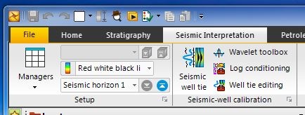
Figure 1: Petrel Seismic well tie button.
2. In the Seismic well tie dialog box that appears, select Sonic calibration from the Study type dropdown list. Select the well or borehole to use (Figure 2).
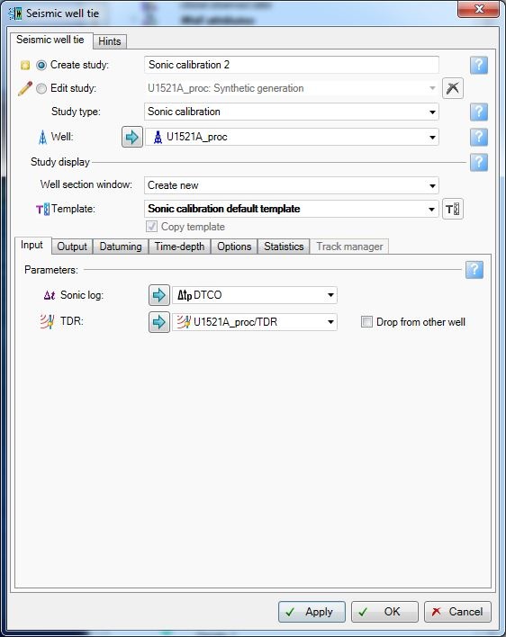
Figure 2: Seismic well tie window configured for creating a new sonic calibration study.
3. For the template field, select the Sonic calibration default template (Figure 2).
Define the parameters in the various tabs at the lower half of the dialogue box. Contextual help or brief description of each parameter is shown if the cursor is moved over the corresponding blue button 
4. Input
In the input tab, select a delta-t compressional or velocity data. The initial TDR can also be a velocity data (stacking, wireline, or laboratory/core) (Figure 2).
5. Output
The two most important output of this calibration process are the Calibrated sonic and TDR. Try to append the default filenames so that you can recognize the output in the Input panel in Petrel. You can also check the "Auto save" box so that all the fine tuning that you will perform will be captured. Alternatively, you can do so only once you are satisfied with the result. The "Set as active TDR" button allows the calibrated TDR to be immediately applied to the well, and can be immediately assessed by opening the interpretation window.
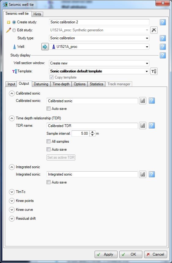
Figure 3: Output tab for seismic well tie window.
6. Datuming
This is one of the most important parameters in executing a seismic well tie. For the sonic velocity through the water column (Vw), a constant value or linear trend is often assumed. However, this is not applicable in deep waters or in proximal offshore where temperature and salinity changes affect the water column velocity. The more accurate Vw can be averaged from the water column sonic profile often used to calibrate side-scan or multibeam bathymetric data, or calculated from the nearest CTD profile using any of the various published empirical equations (e.g., Del Grosso, 1973; Mackenzie, 1981).
For the replacement velocity between the seabed and top-of-log (TOL) (Vb), you can calculate the average velocity from the laboratory measurement of cores should be used (e.g., PWL, PWC).
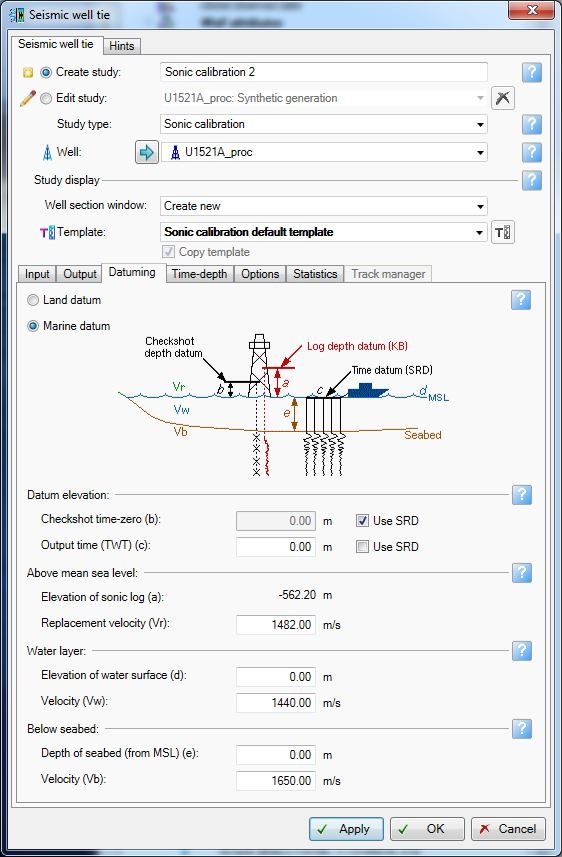
Figure 4: Datuming tab for seismic well tie window, with the different parameters that define a marine datum.
7. Time-depth
The top and bottom of the checkshot data and velocity profile very often do not coincide. In conjunction with the Datuming, this tab provides choices on how checkshots are used above the TOL and below the BOL.
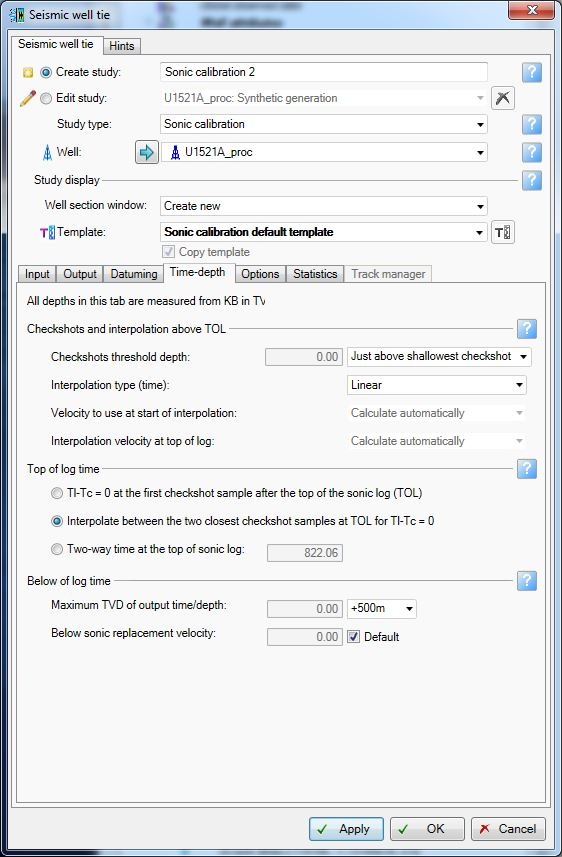
Figure 5: Time-depth tab for seismic well tie window.
8. Options
The user can select how the knee curve is defined in between checkshot or marker points, with the default being a linear trend, but cubic and polynomial fits are also available. the same is true for calculating the residual drift.
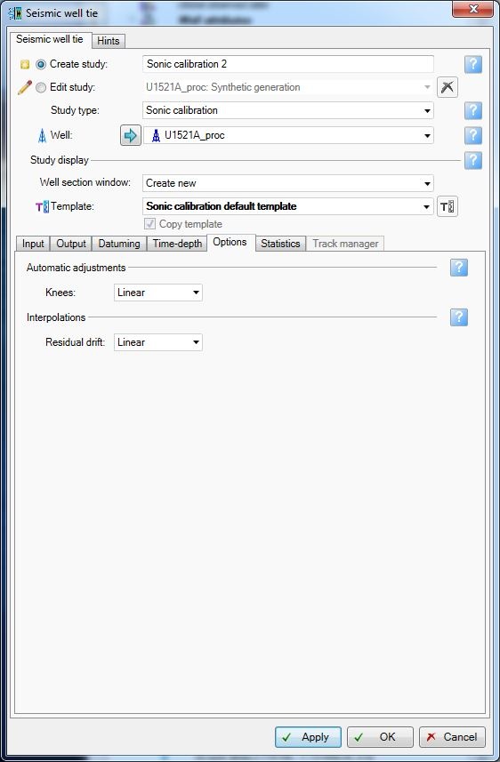
Figure 6: Options tab for the seismic well tie window.
9. When you are satisfied with the parameters, click OK. A well section window will appear showing the results of the calibration process.
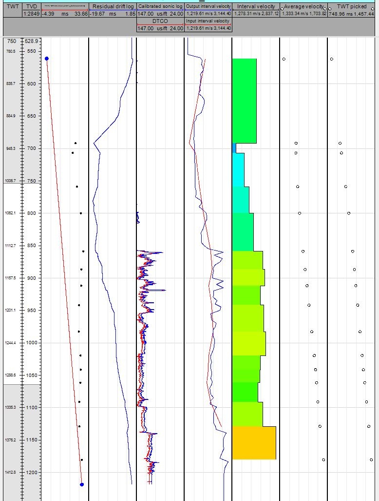
Figure 7: Initial result of the sonic calibration displayed in a well section window.
10. Once the initial sonic calibration output is created, the knee curve can be edited so that the knees can coincide with the checkshot points or to additional locations such as defined well tops. To do this, open the Well tie editing tool palette from Seismic interpretation > Seismic-well calibration group > Well tie editing.
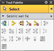
Figure 8: Well tie editing tool palette.
Click on the "Knees at checkshots" button (first row, second from the left button). This will create knees at every checkshot points, as shown below:
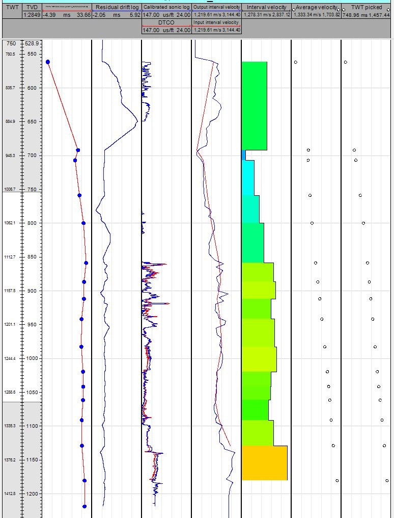
Figure 9: Well section window for sonic calibration with knees at every checkpoint.
11. When satisfied with the outcome of the calibration, go back to the Output tab of the Seismic well tie window and manually or automatically save the calibrated sonic log and apply the calibrated TDR to well.
Credits
This guide is largely derived from the Petrel 2017 Geophysics training manual:
Schlumberger Limited (2018) Petrel 2017 : Petrel Geophysics Workflow/Solutions Training. Houston: Schlumberger, 764 pp.