Introduction
Synthetic seismograms are generated from core or downhole logging data, to emulate or match the corresponding trace in a seismic profile. After the sonic calibration step, generating a synthetic seismogram produces an accurate TDR to increase the confidence in integrating core, logging and seismic profile data.
Procedure
1. Create a new study. In the Seismic interpretation toolbar tab > Seismic-well calibration group > click on the Seismic well tie button (Figure 1).
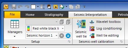
Figure 1: Petrel Seismic well tie button
2. In the window that appears, select Synthetic generation as the Study type, and the name of the well or hole (Figure 2).
In the Input tab:
a) Select a new TDR or use the one currently applied for the well.
b) Choose a wavelet to be convolved with the reflection coefficient, or create a new one by clicking the button to the right of the dropdown box.
c) Identify the seismic profile associated with the well being studied.
d) For calculating the Reflectivity coefficient, the Sonic velocity and density method is often used. Select the logs to be used from the dropdown list, preferably those that have been conditioned and calibrated, especially for the sonic log.
e) Expand the Advanced settings. In cases where the input logs have different depth coverage, there is the option to use only one log by applying the Gardner's equation to generate a synthetic seismogram in the segment that would otherwise be missing.
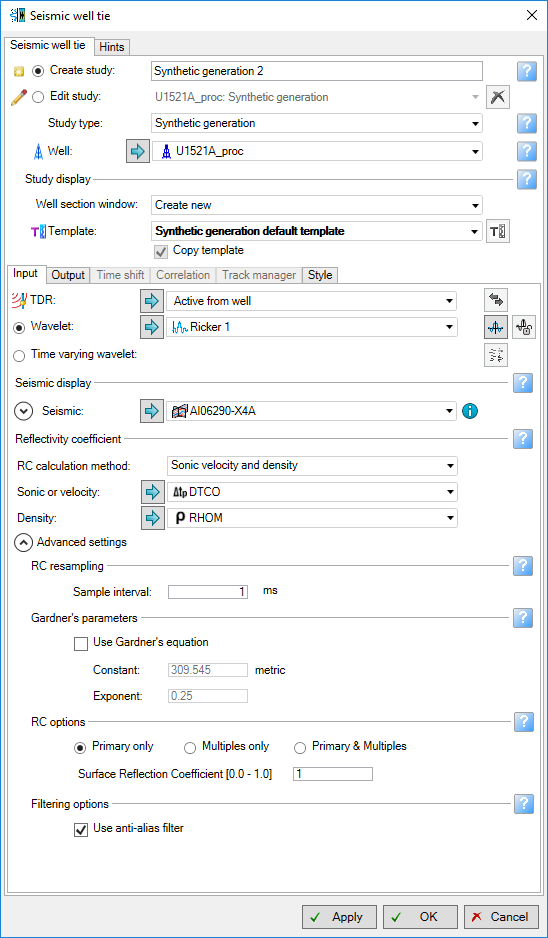
Figure 2: Seismic well tie window configured for generating a new synthetic seismogram.
3. The Output tab, provides the option to save the results of the analysis (Figure 3). Modify or append the default filenames in order to differentiate them from similar logs generated, especially for the TDR (Figure 3).
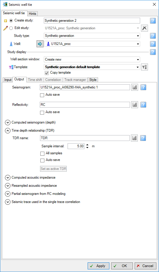
Figure 3: Output tab for the seismic well tie window.
4. Click the Apply button to generate a Well section window displaying the initial synthetic seismogram that is generated (Figure 4).
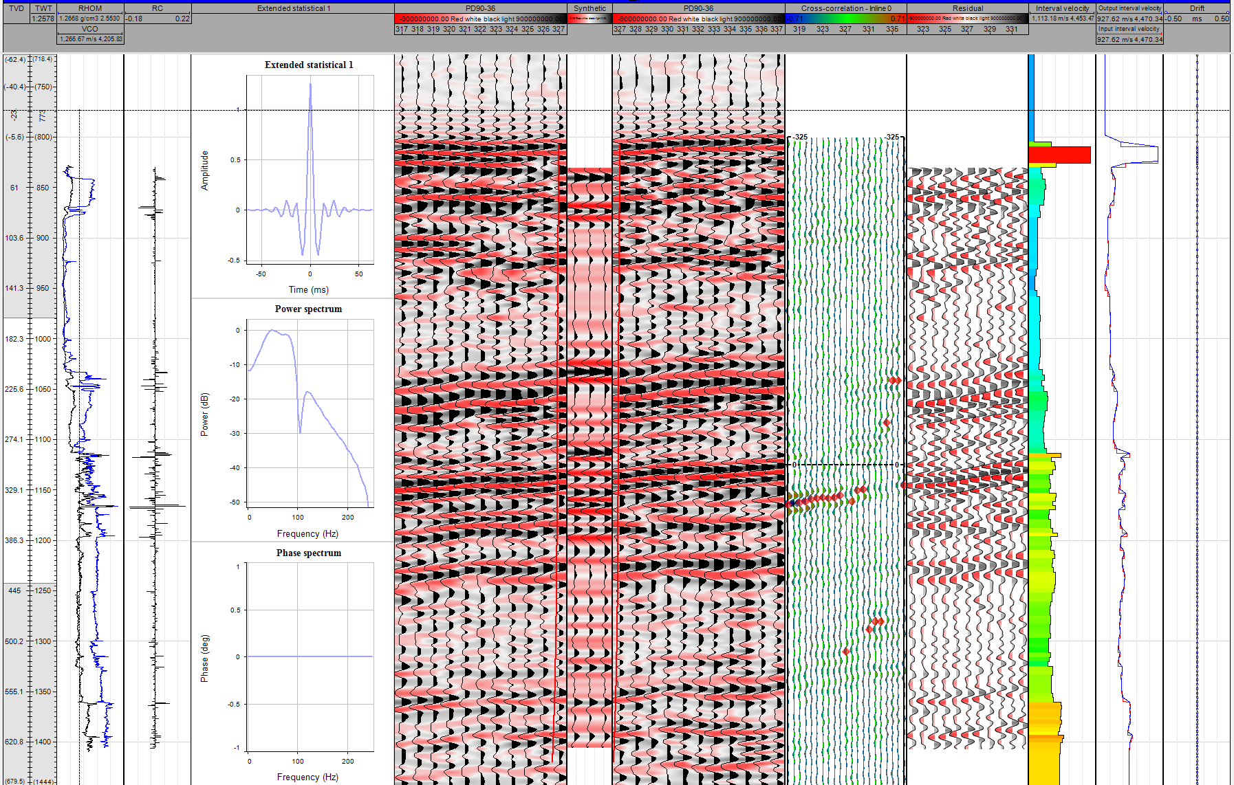
Figure 4: Initial Synthetic seismogram well section window .
5. Refine the resulting synthetic seismogram.
Move the cursor over the Cross-correlation track and, just below the track/column header is a read out indicating the Current position and the Max correlation that can be achieved with the suggested bulk shift to be applied. Take note of these values. The phase shift can later also be included once the phase mistie is computed (see below).
Back in the Seismic well tie window, the remaining tabs for refining the synthetic seismogram are activated.
6. Time shift tab
From the suggested time shift to maximize correlation, enter the value for the bulk shift and check the align box to adjust the vertical position of the synthetic seismogram (Figure 5). Alternatively, this can also be implemented using a button in the Well tie editing toolbar.
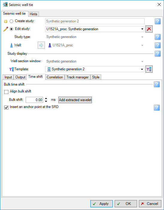
Figure 5: Time shift tab
7. Correlation
The upper (and bottom) segments of a log and a synthetic seismogram are often problematic and should be excluded in the analysis. In calculating the correlation between the synthetic seismogram generated, with a trace or set of traces from the seismic profile, the user can define the start and end time window for the calculation (Figure 6).
In the Trace section, the default is to calculate the correlation to all the seismic traces displayed in the Well section window. Alternatively, the user can define only the trace or a few traces around the actual well/borehole. In a default setting of 10 traces around the well, set the start and end traces to 10 in order to correlate with the only trace corresponding to the well; enter 9 to 11 if the adjacent two traces should be included.
The Phase mistie section in the Correlation tab enables this parameter to be computed. If you hover over a trace in the Correlation track, the readout will show the suggested rotation angle for the wavelet used. To apply this, open the Wavelet toolbox > Phase manipulation tab (Figure 7).
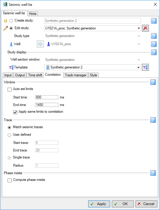 Figure 6: Correlation tab
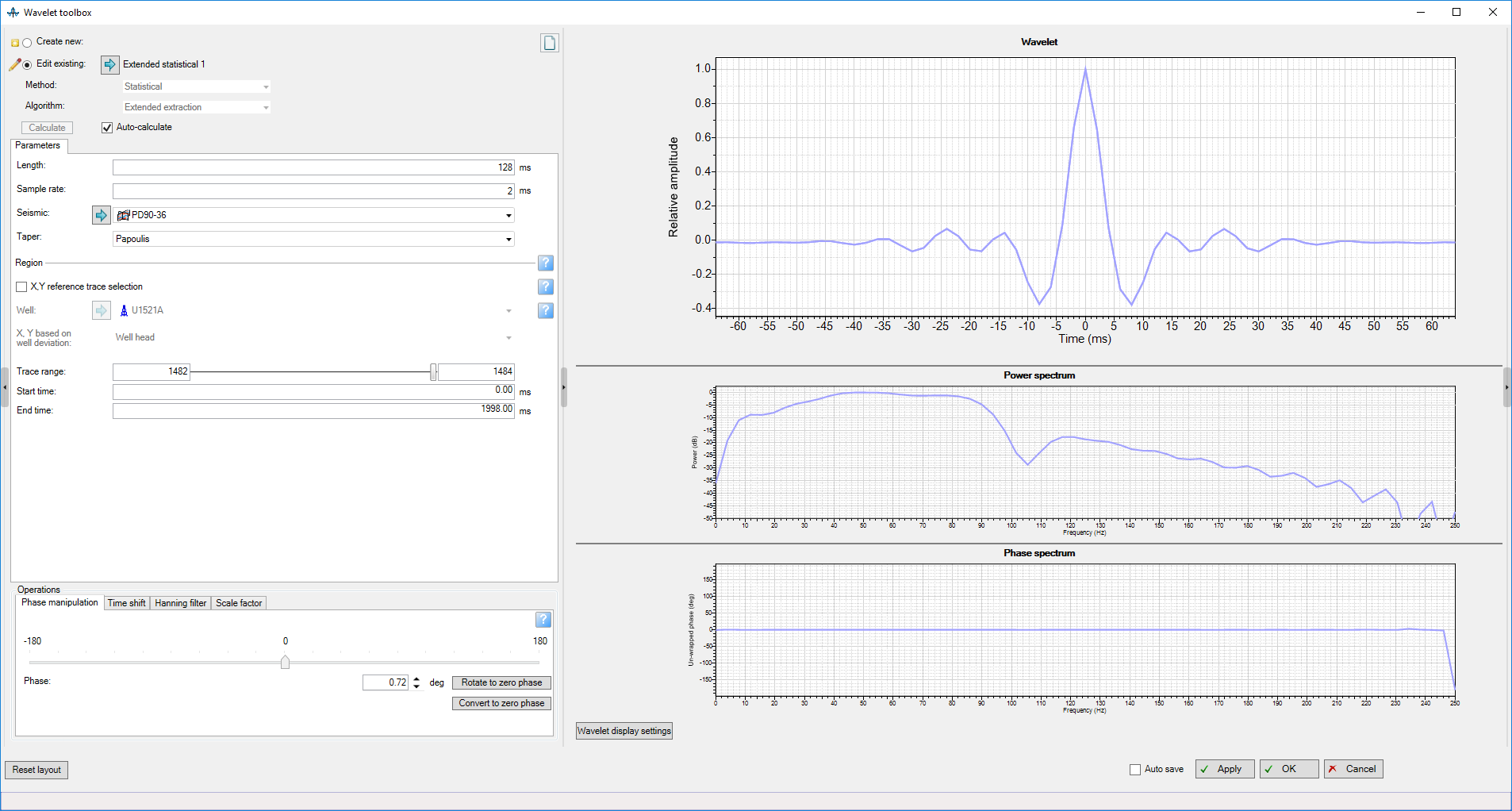 Figure 7: Wavelet toolbox window. In the lower left sector are several adjustable parameters to aid in refining the synthetic seismogram, especially in adjusting the phase.
8. Alignment points
After applying a bulk shift, additional refinement can be made by using alignment points to stretch, squeeze or retain certain segments and horizons of the synthetic seismogram. To perform this process, make sure that the Edit mode is activated in the Well tie editing tool palette window (Figure 7). In either of the seismic trace or synthetic seismogram tracks of the Well section window, click on a prominent reflector, and a green line will appear. Click-and-drag vertically to where you interpret the line should be located. As a good practice, try to limit to no more than 5 strategically positioned alignment points, otherwise, it would imply significant errors in the previous setup or workflows. When you have identified all the alignment points, click on the Align points button in the Well tie editing tool palette window (Figure 8).
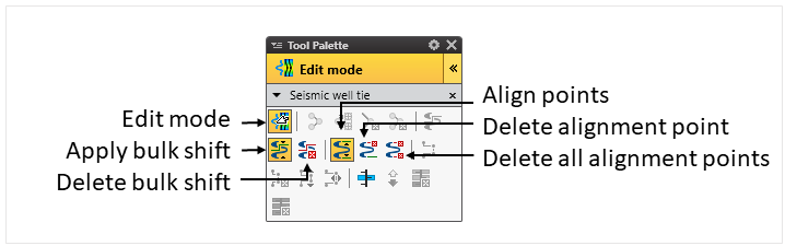
Figure 8: Seismic well tie tool palette
9. Save and apply the results of the analysis.
The final synthetic seismogram well section window is shown in Figure 9. In the Output tab, save and apply the resulting TDR by clicking the corresponding button (Figure 3).
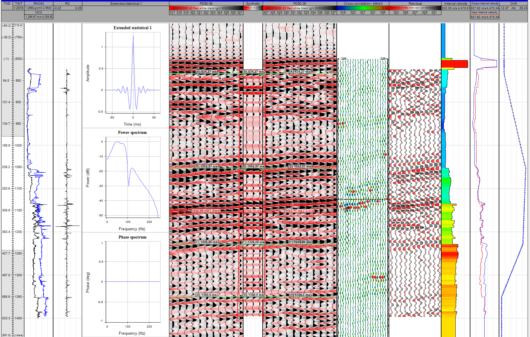
Figure 8: Final Well section window after applying all the bulk time shift and adjustment of alignment points.
Credits
This guide is largely derived from the Petrel 2017 Geophysics training manual:
Schlumberger Limited (2018) Petrel 2017 : Petrel Geophysics Workflow/Solutions Training. Houston: Schlumberger, 764 pp.