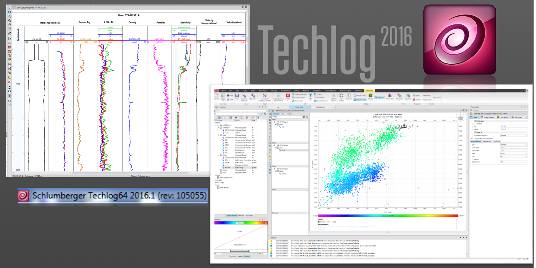
Introduction
This document outlines the steps in creating a basic log and cross-plot of downhole logging data using Techlog. For more advance functionalities, refer to the Techlog Fundamentals Training and Exercise Guide.
A logging dataset is very robust, consisting of many files and hundreds of channels or variables referred to by acronyms, and further multiplied by the different runs and versions (raw and processed). Before starting, please discuss with the Logging Technician and Schlumberger Logging Engineer about the data location and structure. At any point during the plotting process in Techlog, please feel free to consult the Logging Technician for any questions.
Creating a new project from a template
1. Launch Techlog by double clicking on the shortcut icon, either in the desktop or the Windows toolbar (Fig. 1).

Figure 1: Techlog shortcut icon.
2. Once the program opens, familiarize yourself with the basic layout of the Techlog interface, as labelled in Figure 2.
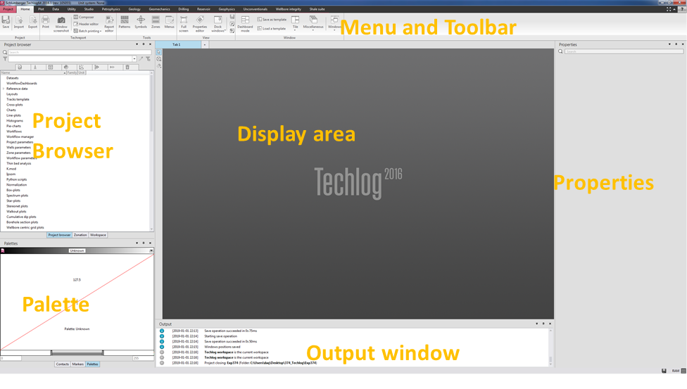
Figure 2: Main components of the Techlog window.
3. On the upper left corner, click on Project > New. A New project window will appear (Fig. 3). Enter a project name (e.g. Exp123) and click Next.

Figure 3: First of four windows that appear in creating a new project.
4. In the second window that appears, select a template project by clicking on the browse button (Fig. 4).
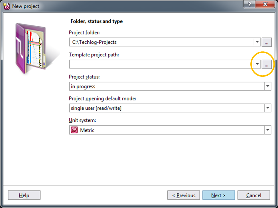
Figure 4: Second of four windows for creating a new project, where a template project is selected.
5. Navigate to C:\Techlog-Projects\IODP-Techlog_template\ and select IODP-Techlog_template.tlp.
6. Skip the third window that appears. In the next (fourth window), click Finish (Fig. 5).
A new project is now created containing a few layout and cross-plot templates used in IODP.
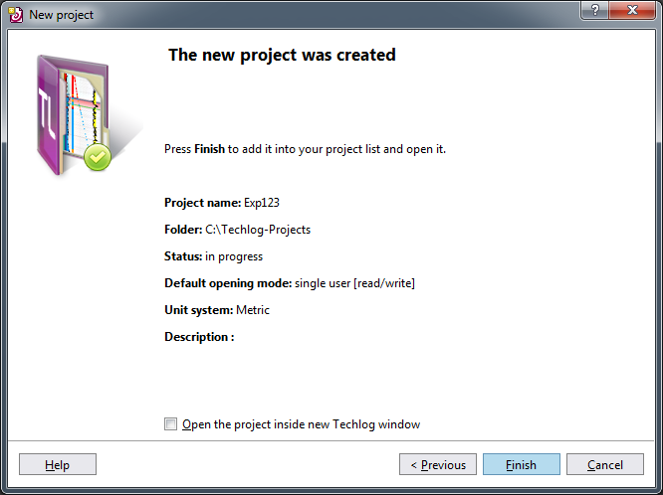
Figure 5: File browser showing the location and IODP-Techlog .
Importing logging data
(Module 2 in Techlog Fundamentals)
Importing DLIS and LAS files
- Under Home menu (upper right), click on the Import button (Fig. 6-1). The Import Buffer panel will appear next to the Project Browser (Fig. 6-2).
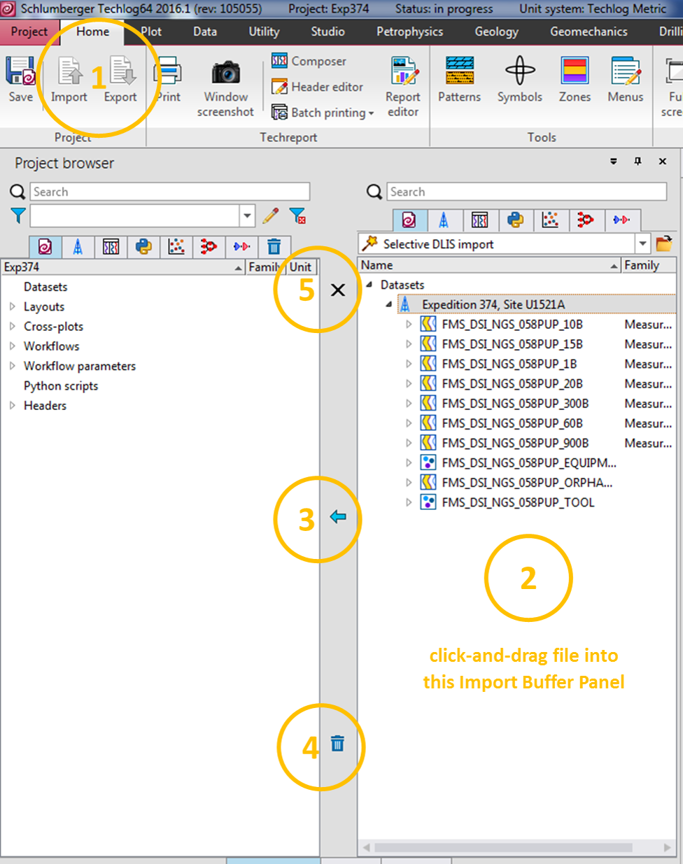
Figure 6: Import Buffer panel.
2. Using Windows File Explorer, navigate to the location of the file that you want to import. Simply click and drag a file to be imported into the Import Buffer panel. Techlog will try to automatically parse the data and select the appropriate import type. The example given in Figure 6-2 is for a DLIS file, which is a generic file type that exists for both raw and processed downhole logging data. The same is true for a LAS file, which is a more streamlined dataset. Consult the Logging Technician or Engineer to identify the files that you may need.
3. Once the data is parsed in the Import Buffer, you can either:
i. Click on the well name (e.g., Expedition 374, Site U1521A), or
ii. click on a particular dataset for that well.
4. To import, click on the blue arrow pointing left (Fig. 6-3).
5. When the progress bar for the import process disappears, click on the bin icon to purge any file in the import buffer (Fig. 6-4).
6. To close the Import Buffer, click on the X icon (Fig. 6-5).
Importing other file types
- Using Windows File Explorer, select a DAT, TXT or CSV file and drag into the Import Buffer Panel (Fig. 7)
- In the Data import wizard window that pops out, define the first line to be imported, the variable name and units (Fig. 7). Use the ASCII file display panel as a reference.
- Click the Preview button.
- Define the variable type for each column. The first column is usually the depth, and is labelled as Reference in Techlog. You also have the option to not import a column (Remove column)
- Click Load to import buffer.
- In the import buffer panel, select the well name and click on the left-pointing blue arrow (Fig. 6-3).
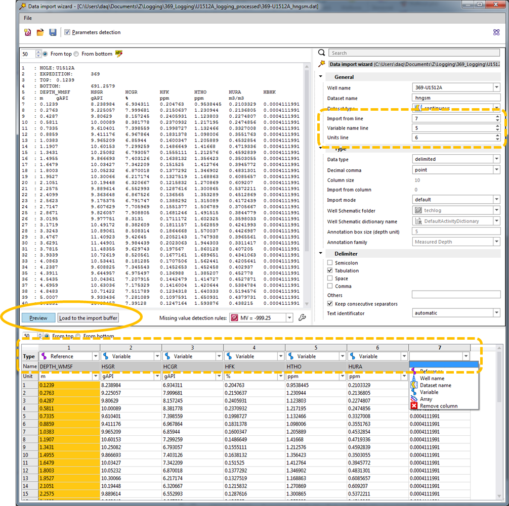
Figure 7: Data import wizard for DAT, TXT and CSV files.
Data management
(Module 3 in Techlog Fundamentals)
After importing a dataset, it is a good practice to browse the different variables to make sure that they have all the parameters required for plotting in Techlog (e.g. family assignment and unit).
- In the Project Browser, expand the Dataset by clicking on the triangle next to it on the left (Fig. 8). The data is arranged in a hierarchy, starting with the well (blue derrick frame icon), dataset (yellow curve icon), and variable (blue curve icon).
2. Click on any of the Dataset items and the corresponding properties will be displayed in the Property panel (see Fig. 2). If the Property Panel is hidden, simply press F4.
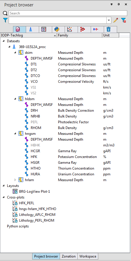
Figure 8: Project Browser panel.
3. Select any of the items in the Dataset and click the right mouse button, and the contextual menu will appear, with the different functions that can be applied (e.g. rename a well as Exp-Site-Hole instead of the default long name given from the source file) (Fig. 9)
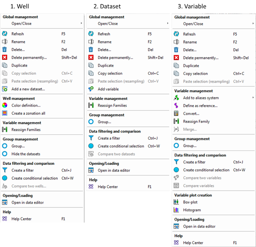
Figure 9: Contextual Right-mouse-button Menu for a well, dataset, and a variable.
4. If any of the dataset variables are grayed-out, it implies that either the family assignment or unit is missing (VS1, VS2, PEFL and HBHK in Fig. 8).
- To assign a Family, RMB click on the variable and select Reassign Families (Fig. 9). If no assignment rules exist for the particular variable, refer to the next section below.
- To define or update the unit designation, refer to the Properties column > Main parameters tab. From the Unit dropdown menu, select the appropriate unit.
5. If the unit is incorrect:
- But the values are correct, simply change the displayed units in the Property panel > Main parameters tab > Unit.
- And the values also need to be converted, RMB-click on the variable and select Convert (Fig. 9-3). In the window that opens, select from the dropdown menu the correct unit.
6. As you are browsing through, you can press the F1 key to invoke the help menu associated with the last selected item in Techlog.
How to create Family assignment rule
1. Click on the Data menu tab (Fig. 10)

Figure 10: Data menu and toolbar, showing the dropdown list for data Families.
2. Click on Family assignment rules.
3. In the window that opens, keep the default selections and click the Reassign families button (Fig. 11).
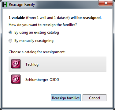
Figure 11: Reassign Family window 1.
4. The Family assignment rules window will appear, showing the list of existing rules. Click on the blue Create new assignment rule button (Fig. 12).
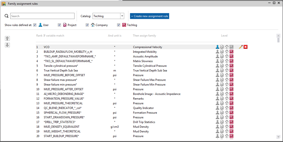
Figure 12: Family assignment rules window.
5. In the Add new assignment rule window that appears (Fig. 13)
i. Select Project.
ii. Type the variable name.
iii. Leave unit as asterisk.
iv. Type in the new family name. A dynamically searching dropdown window will appear from where you can select the actual family name.
v. Click OK
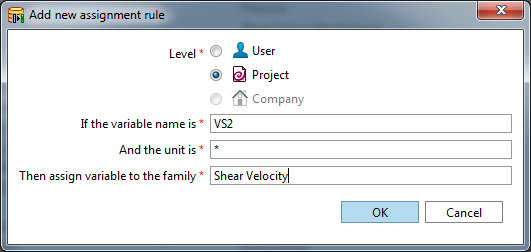
Figure 13: Window for adding new assignment rule.
6.To edit an existing Family assignment rule, simply click on the pencil icon to the far right (Fig. 12).
7. Close the Family assignment rules window shown in Figure 12.
Creating a Log View Plot from a layout template
- In the Project Browser panel, expand Layouts (Fig. 8)
- Double-click on BRG-LogView Plot-1.
- In the Layout template window that appears, select Well template (Fig. 14A).
- A new window will appear for you to select the well to plot, after which, click OK (Fig. 14B).
The Log View Plot will appear in the Display area, as shown in Figure 15.

Figure 14: Pop-out windows for applying a layout template.
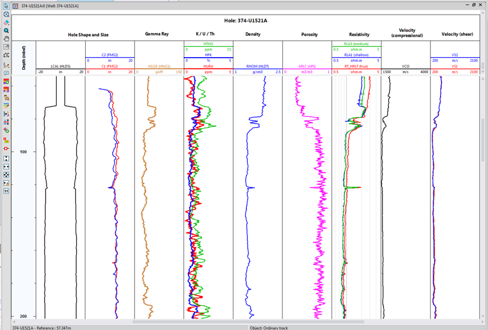
Figure 15: Log View Plot, showing the common variables collected during downhole logging.
Creating a New Log View Plot
- In the Plot menu toolbar, click the LogView button (Fig. 16). A new Log View window will appear in the Display area,
- Select a variable from the Project browser > Dataset. Click-and-drag the variable into the LogView window.
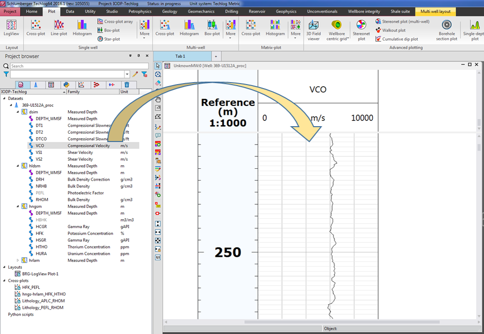
Figure 16: Plot menu toolbar and new LogView plot with a reference (Depth) and variable (VCO) track added.
Editing a Log View Plot
The Techlog Log View plot is very user-interactive. Most of the elements can be selected with the cursor and the corresping properties will appear in the Property panel. The click-and-drag process applies to track boundaries and position. Note however that Undo or Ctrl+Z is almost non-existent in Techlog; you will just have to trace back any edits that you make.
- To expand the window of the Log View Plot, click on the maximize (square icon) button on the upper right corner of the window (Fig. 16)
- If any of the tracks is missing a variable plot, select the associated variable from the Project browser > Dataset and drag it to middle of the designated track.
- To create a new track for a variable, simply click-and-drag a variable in between existing tracks, highlighted as blue columns that temporarily appear in the Log View plot (Fig. 17)
- To edit the appearance of a plot, click on the variable name or line in the header. The line will change to a red dashed line to indicate that it can be edited.
a. In the Property panel, select and update the parameters that you want to edit.
b. To delete a plot, press the Delete button in your keyboard.
5. To change the position of a track, click on the header cell and drag it to the new position.
6. Zooming
a. Press the mouse scroll button and slide the mouse.
b. To zoom on a particular area, select the zoom button (white plus sign inside a green circle) located on the vertical toolbar to the left side of the Log View window. Click-and-drag on the Log View plot.
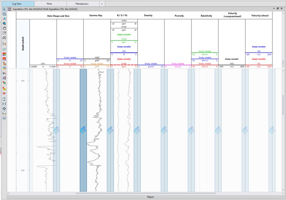
Figure 17: Log View plot in edit mode where the user can drag-and-drop a variable into an existing track, or create a new track in between.
Creating a Cross-plot from a template
- In the Project Browser panel, expand Cross-plots (Fig. 8)
- Double-click on cross-plot template, identified as a scatter-graph icon with a blue paper on the lower right corner.
- In the Layout template window that appears, select Well template (Fig. 14A).
- A new window will appear for you to select the well to plot (Fig. 14B).
A cross-plot will appear in the display area. The example below (Fig. 18) is for Potassium concentration (HFK) on the X-axis and the Photoelectric Factor (PEFL) on the Y-axis, with colors representing standard gamma ray (HSG). Superimposed is the Schlumberger Chart LITH-1A that defines the zones for various clay minerals.
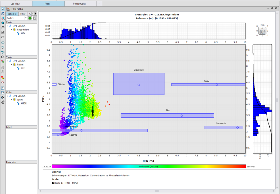
Figure 18: Example of a cross-plot
Creating a new Cross-plot
- In the Plot Menu Toolbar, click on the Cross-plot icon:
- A new Cross-plot window will appear in the Display area (Fig. 19)
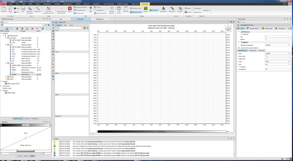
Figure 19: A new Cross-plot window in the Display area.
3. Select a variable from the Datasets and click-and-drag to a corresponding zone in the Variables tab: X axis, Y axis, Color, Label and Point size (Fig. 19)
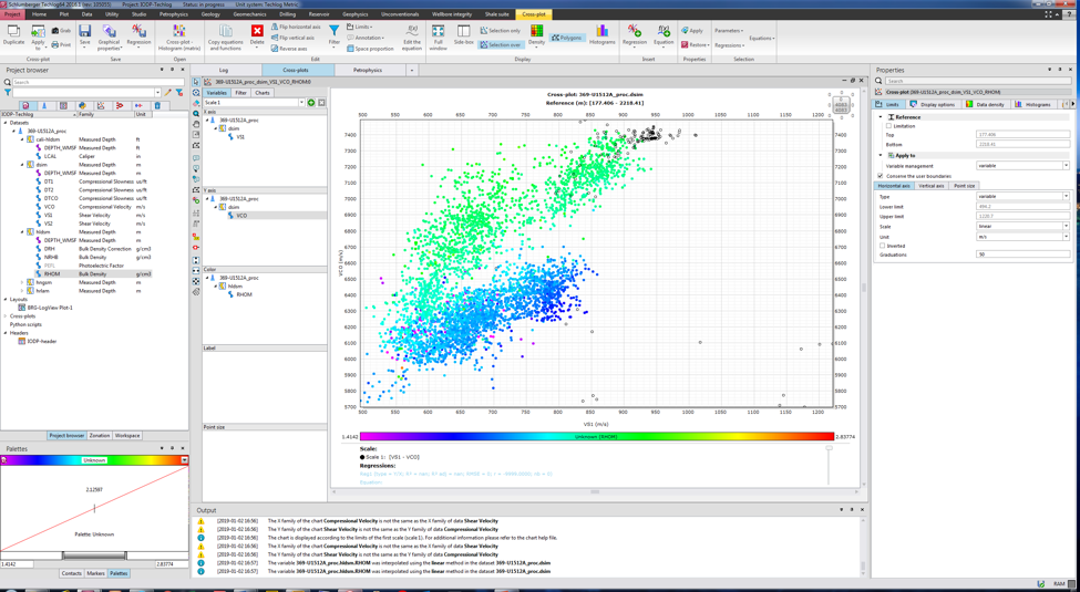
Figure 20: Example of a Cross-plot.
4. Adjust the parameters in the Properties panel. Note that there are several tabs; in case some may be partly hidden, use the left and right arrow button to scroll horizontally.
5. To add a pre-loaded chart, click on the Charts tab left of the cross-plot. A short list of available charts are shown based on the displayed variables. Select one and click the Add button midway down. The selected chart name will be displayed below, and in the actual cross-plot (Fig. 21). In case the chart does not appear, it may be that the dataset is beyond the limits of the chart. Consider adjusting in the Properties panel the limits of the X and Y axis
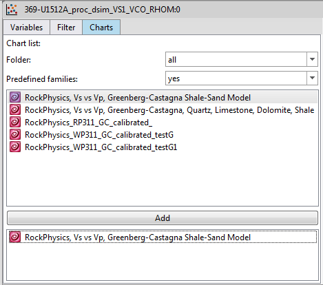 Fig. 21: Cross-plot tab for Charts
Tips
- If the Properties panel is accidentally closed or hidden, (a) simply press the F4 key, (b) click on the Properties editor button in the Home > View toolbar, or (c) Home > Dock windows > Properties.
- By default, some variable log plots (e.g., gamma ray) have a defined baseline and bi-color fill. To remove the baseline and fill, simply click on the filled area in the header, or the baseline boundary in the log plot and click the Delete key on your keyboard.
Credits
This document originated from the Word document Basic_Techlog1_draft1.docx written by Z. Mateo (2019-01-01; see Archived Versions below for a PDF copy). Credits for subsequent changes to this document are given in the page history.
Archived Versions
- Basic Plotting in Techlog 2016 - 27Sept2022
- Basic_Techlog1_draft1.pdf: A PDF version of the original Basic_Techlog1_draft1 written by Z. Mateo, and is superseded by this wiki page.
- BasicPlottinginTechlog2016.pdf - Feb. 24, 2020
