Table of Contents
Introduction
The principles of spectroscopic analysis rely on Beer's law. The principle of Beer's law is that passing light of a known wavelength through a sample of known thickness and measuring how much of the light is absorbed at that wavelength will provide the concentration of the unknown, provided that the unknown is in a complex that absorbs light at the chosen wavelength.
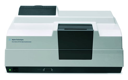
IODP's Agilent Technologies Cary 100 double-beam UV-Vis (ultraviolet–visible) spectrophotometer is ideal for shipboard routine laboratory work. The system measures analytes in interstitial water obtained from sediment cores using standard colorimetric methodology.
Methods
The described methods are based on ODP Technical Note 15, Chemical Methods for Interstitial Water Analysis Aboard the JOIDES Resolution, Aug 1991; J.M. Gieskes, T. Gamo, and H. Brumsack.
Ammonium
Determination of ammonium concentration is of importance because this constituent is an indicator of diagenesis of organic matter in the sediments. The onset of sulfate reduction coincides with initiation of ammonium ion production. Ammonium production increases strongly in the zone of methanogenesis, presumably as a result of associated deammonification reactions. The large potential variation in ammonium concentrations, therefore, suggests that a few preliminary ammonium concentrations should be run in order to set limits to the sample dilution and range of standards to be used. Suggestions for this follow below.
The methodology is based on Solorzano (1969), originally developed to detect very small NH4+ concentrations in seawater. Although background contamination problems in seawater are enormous, the relatively high concentrations of ammonium in pore fluids (as high as 85 mM in ODP Leg 112 samples; Kastner et al., 1990) minimizes this problem when matrix blanks are run along with the samples. In areas of low sedimentation, however, very low ammonium concentrations require careful sample handling to avoid this problem.
The ammonium method is based on diazotization of phenol and subsequent oxidation of the diazo compound by Chlorox™ to yield a blue color, measured spectrophotometrically at 640 nm.
Reagent Solutions
A: 95% Ethanol (100 mL) – make fresh daily
B: Phenol solution (101 mL) – make fresh daily
Dissolve 1 mL of liquid phenol in Reagent A. Note: phenol is highly toxic and appropriate care should be taken.
C: Sodium Nitroprusside solution (100 mL) – make fresh daily
Dissolve 75 mg of sodium nitroprusside (Na2[Fe(CN)5NO]) in 100 mL nanopure water.
D: Alkaline solution (500 mL) – make fresh monthly
Dissolve 7.5 g trisodium citrate tribasic dihydrate (Na3C6H5O7·2H2O) and 0.4 g sodium hydroxide (NaOH) in 500 mL nanopure water.
E: Oxidizing solution (51 mL) – make fresh daily
Dissolve 1 mL fresh sodium hypochlorite (4% available chlorine) in 50 mL Reagent D. Note: Use sodium hypochlorite or regular strength Chlorox™ bleach. DO NOT use Chlorox that contains NaOH, fragrances, or other agents, and do not use another brand of bleach.
F: Ammonium standard: 0.10 M Ammonium (1000 mL) – make fresh monthly
Dry ammonium chloride (NH4Cl) overnight in an oven.
Dissolve 5.345 g dried NH4Cl in nanopure water; bring to 1000 mL in a volumetric flask.
Standards
50 mL batches are stable for 1 month. (Note that the 50 µM solution is prepared from the 1000 µM standard, and the rest of the standards are made from the 100 mM primary stock standard.)
concentration (µM) | volume of nanopure water (mL) | volume of ammonium standard (mL) | note |
|---|---|---|---|
0 | 50.00 | 0 |
|
50 | 47.50 | 2.50 | (dilute from 1000 µM std) |
100 | 49.95 | 0.05 | (dilute from 100 mM std) |
200 | 49.90 | 0.10 | (dilute from 100 mM std) |
400 | 49.80 | 0.20 | (dilute from 100 mM std) |
600 | 49.70 | 0.30 | (dilute from 100 mM std) |
800 | 49.60 | 0.40 | (dilute from 100 mM std) |
1000 | 49.50 | 0.50 | (dilute from 100 mM std) |
1500 | 49.25 | 0.75 | (dilute from 100 mM std) |
2000 | 49.00 | 1.00 | (dilute from 100 mM std) |
3000 | 48.50 | 1.50 | (dilute from 100 mM std) |
Procedure
Concentrations of ammonium may differ quite a bit at different sites. Typically in areas with strong evidence of organic carbon diagenesis (e.g., organic carbon–rich sediments), high concentrations of NH4+ can be expected. In that case, sample aliquots must be made appropriately small or sample dilution may be required. The range can be established by using a sample near the alkalinity maximum. Once the range has been determined, prepare standards that cover this range. In this manner, samples and standards are treated in a similar way.
The high range of the instrument is 3.0 absorbance units (Abs). The results are linear up to this point. If the readings are expected to be higher than 3.0 Abs, use a sample volume of 30 µL instead of 100 µL and divide measured concentrations by 0.3 to arrive at the final sample concentration.
Care should be taken to use clean vials, preferably not those used for Si and PO4 determinations, in which ammonium molybdate is used as a reagent.
Note:
The order of dilution (below) matters, so do not change this order.
Shake samples after EACH addition.
- Transfer 200 µL of sample/standard to an 8 mL vial.
- Add 2 mL of nanopure water to each vial and shake.
- Add 1 mL phenol-alcohol solution to each vial and shake.
- Add 1 mL sodium nitroprusside to each vial and shake.
- Add 2 mL of oxidizing solution to each vial and shake.
Let the color develop (in a dark place) for 6.5 hr* and then determine the absorbance at 640 nm wavelength.
*(from a series of measurements over 8 h, it was found that results stabilized after 6.5 hr.)
Phosphate
Determination of dissolved phosphate, particularly in rapidly deposited organic carbon–rich sediments, is important in the shipboard analytical program. Phosphate concentrations may vary considerably, and it is therefore advisable to obtain a preliminary idea of the concentration ranges to be expected. This can most easily be accomplished by taking samples in the region of maximum alkalinities. Typically if alkalinities are >30 mM, dissolved phosphate concentrations may be >100 µM; thus, only very small sample aliquots will be needed to establish the concentration range.
This method is, in essence, the colorimetric method from Strickland and Parsons (1968) as modified by Presley (1971) for DSDP pore fluids. Orthophosphate reacts with Mo(VI) and Sb(III) in an acidic solution to form an antimony-phosphomolybdate complex. Ascorbic acid reduces this complex to form a blue color, and absorbance is measured spectrophotometrically at 885 nm.
It is important to note that the concentrations in the final test solution cannot exceed ~10 µM. Thus, for open-ocean (low sedimentation rate, low organic carbon) sediments, one might need to do the determination on 2 mL of sample (expected range 0–10 µM), but in typical continental margin settings, where concentrations can exceed 100–200 µM, a 0.1 or 0.2 mL sample aliquot must be used. The concentration range must be established prior to running samples, and it is highly advisable to make standards that cover the range of concentrations to be expected.
Note: Samples with high silica concentrations may give a false increase in measured concentration of phosphate (http://dx.doi.org/10.1007/BF02071829; S. Noriki, Silicate correction in the colorimetric determination of phosphate in seawater, 1983).
Reagent Solutions
A: Sulfuric Acid solution (H2SO4) (1000 mL) – stable indefinitely
While stirring, carefully add 10 mL concentrated H2SO4 to ~ 600 ml nanopure water in a 1000 ml volumetric flask. CAUTION: Mixing sulfuric acid and water produces heat. Take appropriate precautions.) Allow to cool to room temperature before diluting to 1000 mL with nanopure water.
B. Antimony Potassium Tartrate solution (1000 mL) – make fresh every two months; store in amber glass @ 4°C
In a 1000 mL volumetric flask, dissolve 0.102 g of antimony potassium tartrate trihydrate (KSbC4H4O7·3H2O) in ~ 600 mL of nanopure water. (If using antimony potassium tartrate hemihydrate [KSbC4H4O7·½H2O], dissolve 0.09 g.) Dilute to 1000 mL with nanopure water.
C. Ammonium Molybdate solution (1000 mL) – stable indefinitely; store in polyethylene @ 4°C
In a 1000 mL volumetric flask, dissolve 2 g of ammonium molybdate tetrahydrate ([NH4]6Mo7O24·4H2O) in ~ 600 mL of nanopure water. Dilute to 1000 mL with nanopure water.
D. Ascorbic Acid solution (1000 mL) – make fresh every week; store in amber glass @ 4°C
In a 1000 mL volumetric flask, dissolve 3.5 g of ascorbic acid (C6H8O6) in ~ 600 mL nanopure water. Dilute to 1000 mL with nanopure water. Note: If the reagent is discolored upon creation, the dry ascorbic acid is probably oxidized and must be replaced.
E. Mixed reagent (250 mL) – make fresh every 6 hours
Add the following solutions to an appropriate container. Do not add the ascorbic acid reagent until immediately before use.
Mix well after each addition to prevent the solution from darkening.
solution | volume (mL) |
Ammonium molybdate (Reagent C) | 50 |
Sulfuric acid (Reagent A) | 125 |
Antimony potassium tartrate (Reagent B) | 25 |
Ascorbic acid (Reagent D) (immediately before use) | 50 |
F. Primary standard: 0.01 M Phosphorus (1000 mL) – make fresh every 4 weeks; store @ 4°C
Dry monobasic potassium phosphate monobasic (KH2PO4) in oven at 100°C for two hours; keep in a desiccator while it cools before weighing.
In a 1000 mL volumetric flask, dissolve 1.361 g oven-dried KH2PO4 in ~ 600 mL nanopure water, then dilute this solution to 1000 mL with nanopure water.
Standards
concentration (µM) | volume of primary standard (mL) | volume of nanopure water (mL) |
|---|---|---|
0 | 0 | 100 |
5.0 | 0.050 | 99.95 |
10.0 | 0.100 | 99.90 |
15.0 | 0.150 | 99.85 |
20.0 | 0.100 | 49.90 |
40.0 | 0.200 | 49.80 |
60.0 | 0.300 | 49.70 |
80.0 | 0.400 | 49.60 |
100 | 0.500 | 49.50 |
200 | 1.000 | 49.00 |
300 | 1.500 | 48.50 |
Procedure
- Add 2 mL nanopure water to a 8 mL vial.
- Add 600 µL sample or standard.
- Add 4 mL mixed reagent.
- Shake well.
After a few minutes a blue color develops, which remains stable for a few hours. It is best to make the readings at 885 nm ~ 30 min after addition of the mixed reagent.
Note: Use a smaller aliquot of sample if the result exceeds the linear range of the spectrophotometer, making up the volume with nanopure water. (For example, for a 300 µL aliquot of a sample, add 300 µL nanopure water.)
Silica
Silicon is routinely measured on the ICP, so measurement by spectroscopic analysis can be considered an alternate method.
Dissolved silica determinations are of great importance in interstitial waters. Often they represent the lithology of the sediments, and the concentrations can vary substantially, especially if highly dissolvable phases such as biogenic opal-A, volcanic ash, or smectite are present. Thus, a wide range of concentrations can be expected, typically from 50 to 1200 µM or higher (especially in hydrothermally affected sediments). The method below usually covers the range, although greater dilutions may be appropriate if sediments or sample sizes necessitate this.
This method is based on the production of a yellow silicomolybdate complex. The complex is reduced by ascorbic acid to form molybdenum blue, measured at 812 nm. The blue complex is very stable, which will enable delayed reading of the samples.
Reagent Solutions
A: Sulfuric Acid stock solution (500 mL) – make fresh every month; store in polyethylene
Slowly pour 250 mL of concentrated sulfuric acid into a 500 mL volumetric flask containing ~ 200 mL of nanopure water. (Caution: Mixing concentrated sulfuric acid and water produces heat. Take appropriate precautions.)
Allow to cool to room temperature before diluting to 500 mL with nanopure water.
B. Ammonium Molybdate Tetrahydrate solution (500 mL) – make fresh every month; store in dark polyethylene @ 4°C
In a 500 mL volumetric flask, dissolve 4 g of ammonium molybdate tetrahydrate ((NH4)6MO7O24·4H2O) in ~300 mL of nanopure water. Add 12 mL of concentrated hydrochloric (HCl) acid, mix, and make up to 500 mL with nanopure water. Note: If a white precipitate forms, make fresh reagent.
C: Metol Sulfite solution (500 mL) – make fresh every month; store in amber glass, tightly sealed @ 4°C
Dissolve 6.0 g anhydrous sodium sulfite, Na2SO3, in a 500 mL volumetric flask. Add 10 g Metol (p-methylaminophenol sulfate [(C7H10NO)2SO4]) and then nanopure water to make the volume to 500 mL. When the Metol has dissolved, filter the solution through a Whatman No. 1 filter paper. Note: This solution may deteriorate quite rapidly.
D: Oxalic Acid solution (500 mL) – make fresh every month; store in glass
In a 500 mL volumetric flask, shake 50 g of analytical-grade oxalic acid dihydrate [(C2H4O2)·2H2O] in ~ 300 mL of nanopure water. Shake well and bring to 500 mL. Let stand overnight. Decant saturated solution of oxalic acid from crystals before use.
E: Reducing solution (150 mL) – make fresh daily
Mix 50 mL reagent C (Metol solution) with 30 mL reagent D (oxalic acid solution). Add slowly, with mixing, 30 mL reagent A (50% sulfuric acid solution) and bring volume to 150 mL with nanopure water.
F: Synthetic seawater (1000 mL) – make fresh monthly; store in polyethylene
In a 1000 mL volumetric flask dissolve 25 g sodium chloride in ~ 800 mL nanopure water, then add 8 g magnesium sulfate heptahydrate (MgSO4·7H2O). Dilute to 1000 mL with nanopure water.
G. 3000 µM Silica Primary Standard (1000 mL) – make fresh every 2 months; store in polyethylene
Note: When sodium silicofluoride (Na2SiF6) is dissolved in water, it hydrolyzes to form reactive dissolved silica. Place ~ 1 g of Na2SiF6 in an open vial and place in a vacuum desiccator overnight to remove excess water. Do not heat.
In a 1000 mL polyethylene volumetric flask, dissolve 0.5642 g dried sodium silicofluoride in ~ 800 mL nanopure water. Dissolution is slow; allow at least 3 minutes. Dilute the solution to 1000 mL with nanopure water.
Standards
Using a 50 mL volumetric flask, add the following amounts of primary standard to approximately 30 mL of nanopure water and then bring to a total of 50 mL. Store in polyethylene containers.
concentration (µM) | volume of primary standard (mL) | volume of nanopure water (mL) |
30 | 0.5 | 49.5 |
60 | 1.0 | 49.0 |
120 | 2 | 48.0 |
240 | 4 | 46.0 |
360 | 6 | 44.0 |
480 | 8 | 42.0 |
600 | 10 | 40.0 |
900 | 15 | 35.0 |
1200 | 20 | 30.0 |
Procedure
Make sure that all reagents are prepared ahead of time. The method has a time factor built in, and therefore it is of great importance to have all necessary reagents ready to go.
- Pipette 4 mL of nanopure water into the vials (3.8 mL for standards and blanks).
- For standards and blanks (nanopure water), pipette 200 µL of synthetic seawater into the vials.
- Pipette 200 µL of sample/standard/blank into the vials.
- Record time.
- Add 2 mL of molybdate solution (reagent B) to the vials. A yellow color will develop; allow to mature for exactly 15 minutes (± 15 s).
- Add 3 mL of the reducing solution (reagent E).
- Cap the vials and let stand for at least 3 hours.
- Read absorbances on the spectrophotometer at 812 nm.
Procedure notes
- Do not handle more than about thirty samples at a time in order to ensure that the 15 min time limit can be adhered to. Make sure that there are no large fluctuations in room temperature.
- Do not use synthetic seawater in dilutions of the primary standard. This could cause the decrease in reactive silica in a few hours as a result of polymerization reactions.
- The reason for adding 200 µL of synthetic seawater to the standards is to maintain a reasonably uniform salt content in relation to the samples, this suppressing a potential salt effect on the method.
- It is important to wait at least three hours for the blue color to develop; the higher the concentration, the longer the time. The color remains stable for many hours, and reading after 4–5 hours may, in fact, be a good idea. Again, consistency in time limits is advisable.
Sulfide
The sulfide method is based off a method developed by Cline in 1969. This method called for very large volumes of water (50 mL). This method was modified on the BONUS Baltic Gas expedition in 2011 to work with sample volumes in the 1-5mL range.
The method is a bit tricky in that the reagent concentrations change depending on what concentration range your samples fall in:
- High range: 6-80 uM
- Low range: 1-10 uM.
All samples need to be preserved during splitting with a 1% zinc acetate solution. It can require a relatively large amount of sample in order to do this analysis. The high range method uses less sample (~500 µL), but if the sulfide level is below 6 µM, it won't be enough. It may still be worth screening samples with the high-range method in order to conserve interstitial water sample volume. The low-range method requires 4 mL (8x the amount of sample) but is sensitive down to 1 µM. The scientists will have to determine if consumption of 4 mL, possibly 4.5 mL, of sample is worth obtaining the sulfide concentration.
Reagent Solutions
A: 1% zinc acetate (w/v)
For Standard: Prepare 1 L of 1% zinc acetate by dissolving 10 g zinc acetate dehydrate into about 600 mL DI water in a 1 L volumetric flask. Add 1 mL of concentrated acetic acid, bring up to volume, and mix well.
For Splits: Prepare 100 mL of 1% zinc acetate by dissolving 1.0 g zinc acetate dehydrate into about 60 mL DI water in a 100 mL volumetric flask. Add 100 µL of concentrated acetic acid, bring up to volume, and mix well.
B: 1 mM zinc-sulfide standard suspension
Before weighing the sodium sulfide nonahydrate, wash the crystals off with nanopure water and dry with a clean Kim Wipe to remove the oxidation products from the crystal before weighing. Try to select very small crystals (or break them up) to facilitate accurate weighing. Dissolve 0.20 g of Na2S·9H2O in 1 L of 1% zinc acetate solution (Reagent A). Store in plastic and cool. Shake vigorously each time before using.
Note: It is very difficult to weigh 0.20 g of this reagent accurately because of the size of the crystals. Weigh 0.20 g within 5 mg and then record the mass used on the bottle. The Baltic Gas methods paper (Ferdelman et al., 2011) describes the use of sodium thiosulfate to standardize the Zn-S suspension, but this has not been the standard practice.
C: 100 µM zinc-sulfide standard
Dilute 10 mL of 1 mM zinc-sulfide standard suspension (Reagent B) up to 100 mL with nanopure water. This is the stock standard for the dilution of the standard curve.
D: High-Range Sulfide Diamine Reagent
For the high-range (6-80 µM) method, add 500 mL of concentrated HCl to 500 mL of nanopure water. Mix thoroughly and allow to cool to room temperature. Add 4.0 g of N,N-dimethyl-p-phenylenediamine sulfate and 6.0 g iron chloride hexahydrate (FeCl3·6H2O), mix well, and refrigerate in an amber Nalgene bottle.
E: Low-Range Sulfide Diamine Reagent
For the low-range (1-10 µM) method, add 250 mL of concentrated HCl to 250 mL of nanopure water. Mix thoroughly and allow to cool to room temperature. Add 0.50 g of N,N-dimethyl-p-phenylenediamine sulfate and 0.75 g iron chloride hexahydrate (FeCl3·6H2O), mix well, and refrigerate in an amber Nalgene bottle.
F: Dilution Reagent
This reagent is used to dilute too-dark samples into the range of color covered by the standard curve, while keeping a constant concentration of the diamine reagent. Create this reagent as appropriate for the high-range or low-range method:
For the high-range method, add 800 µL of Reagent D to 10 mL of nanopure water.
For the low-range method, add 4 mL of Reagent E to 50 mL of nanopure water.
Sample Preservation
The IW splits for sulfide should be preserved immediately with the 1% zinc acetate solution (Reagent A) to prevent the loss of dissolved sulfide.
- For 0.5 mL aliquots (high range method), fix the sulfide with 40 µL of 1% zinc acetate.
- For 4.0 mL aliquots (low-range method), fix the sulfide with 800 µL of 1% zinc acetate solution.
Procedure
High-Range Method
Make dilutions of the 100 µM zinc-sulfide standard (Reagent C) for the standards to create 0.5 mL of standard at each level.
standard level | reagent C ( µL) | nanopure water (µL) | concentration (µM) |
blank | 0 | 500 | 0.0 |
6 | 30 | 470 | 6.0 |
20 | 100 | 400 | 20 |
40 | 200 | 300 | 40 |
60 | 300 | 200 | 60 |
80 | 400 | 100 | 80 |
- Well shake the zinc acetate-preserved sample
- Pipette the sample (0.5 mL) into the vial.
- Add 40 µL of the high-range diamine reagent (Reagent D) to the sample, blank, and standards and shake each vial.
- Place the samples, blank, and standards, into the dark for 30 minutes. The standards should turn blue. If the visual appearance of any of the samples is darker blue than the highest standard, dilute the sample in the dilution reagent (Reagent F) until it is within the color range of the standards.
Low-Range Method
Make dilutions of the 100 µM zinc-sulfide standard (Reagent C) for the standards to create 4 mL of standard at each level. Add the specified volume of Reagent C and nanopure water as shown in the table below to create the standards.
concentration (µM) | reagent C (µL) | nanopure water (µL) |
0 | 0 | 4000 |
1 | 40 | 3960 |
2.5 | 100 | 3900 |
5 | 200 | 3800 |
7.5 | 300 | 3700 |
10 | 400 | 3600 |
- Well shake the zinc acetate-preserved sample.
- Pipette the sample (4 mL) into the vial.
- Add 320 µL of the low-range diamine reagent (Reagent E) to the sample, blank, and standards, and shake each vial.
- Place the samples, blank, and standards into the dark for 30 minutes. The standards should turn blue. If the visual appearance of any of the samples is darker blue than the highest standard, dilute the sample in the dilution reagent (Reagent F) until it is within the color range of the standards.
Note: From the Exp. 366 Methods chapter
Hydrogen sulfide (expected to be HS- at the pH of most IW samples) concentrations were analyzed following the method of Cline (1969) with modifications as adapted for small volumes of pore fluids by Ferdelman et al., 2011. Initially, 500 µL sample was fixed with 40 µL of a 1% zinc acetate solution, and reagents used were for a range of 6 to 80 µM. However, because most samples were below detection for the first set of samples, 4 ml sample was fixed with 800 µL zinc acetate solution, and the analyses were conducted following the lowest range (1 to 3 µM) outlined in Cline (1969), which had a linear range for the calibration curve at least up to 10 µM. The zinc acetate fixed sample was vigorously shaken and 320 µL of a diamine solution consisting of 0.5 g N,N-dimethyl-p-phenylenediamine sulfate and 0.75 g ferric chloride (FeCl3 * 6H2O) per 500 ml nanopure water, was added. The solution was shaken, and left for 30 minutes in the dark, then measured by spectrophotometry at 670 nm. If the blue color of the sample was visually darker than that of the highest calibration standard (10 µM), the sample was diluted with nanopure water until a lighter color was observed.
Analyzing Samples
Preparing the Cary Spectrophotometer
- Engage the tubing on the peristaltic pump. Make sure that the waste line goes into a receptacle.
- Turn on the unit and let it warm up for at least three hours at the wavelength in question.
- Confirm that the instrument Beam Mode is correctly configured.
- In Varian > Cary WinUV start the Advanced Read application.
- Click the Setup button and select the Options tab.
- Confirm in the Beam Mode area that Double Beam is selected and Normal is also selected.
- Confirm in the Beam Mode area that Double Beam is selected and Normal is also selected.
SPS3 Autosampler
The Agilent Technologies SPS3 autosampler facilitates sample introduction into the Cary Spectrophotometer with minimal operator interaction.
The SPS3 is connected to the PC via a RS232 cable to a Keyspan USB converter and the SPS3 is connected to the Cary unit via a RSA sample inlet tube (Figure 1).
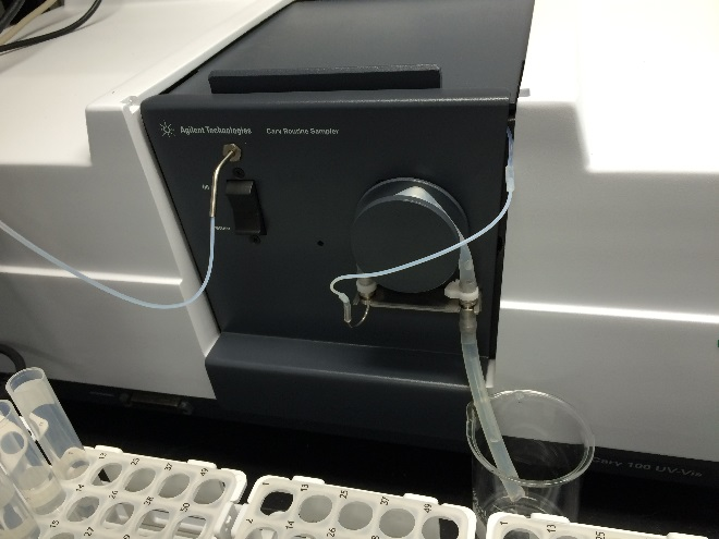

Figure 1 : Sample inlet tube and flow cell
The reservoir peristaltic pump (Figure 2) allows nanopure water to be pumped through the system between samples to flush lines. Pump speed is controlled by a dial above the pump. This pump fills the reservoir but does not change the flow into the Cary's flow cell; that is controlled by the spectrometer's peristaltic pump.
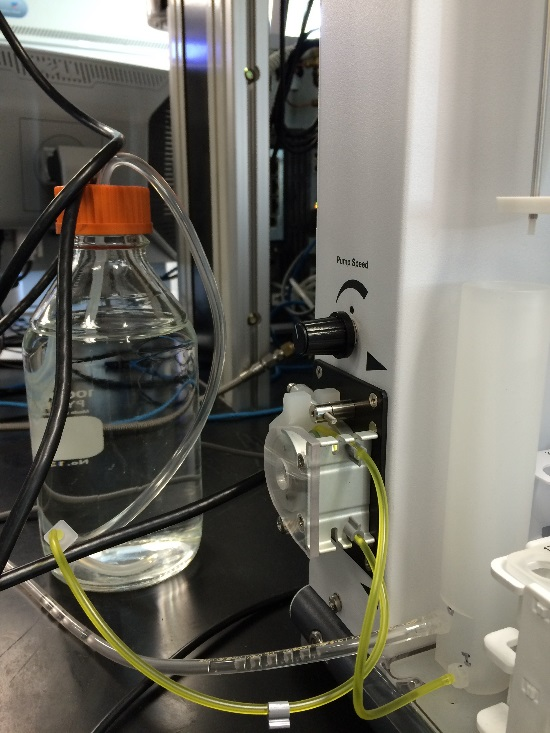
Figure 2 : SPS3 Reservoir peristaltic pump
Sample trays allow up to 180 samples to be run (Figure 3). First vial is a "zero" (nanopure water).
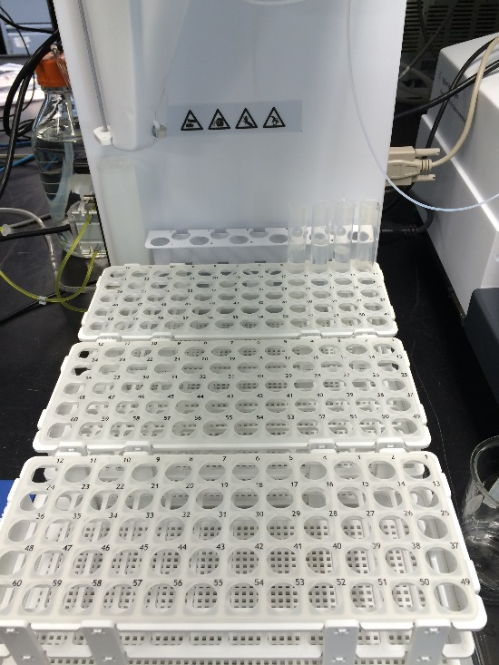
Figure 3 : SPS3 Sample trays
Software setup
Advanced Reads setup

Figure 4 : Advanced Reads main screen

Figure 5 : Setup (Entering sample information)

Figure 6 : Setup (Sipper settings [Cary peristaltic pump])

Figure 8 : Setup (Rinse/Sample trays)
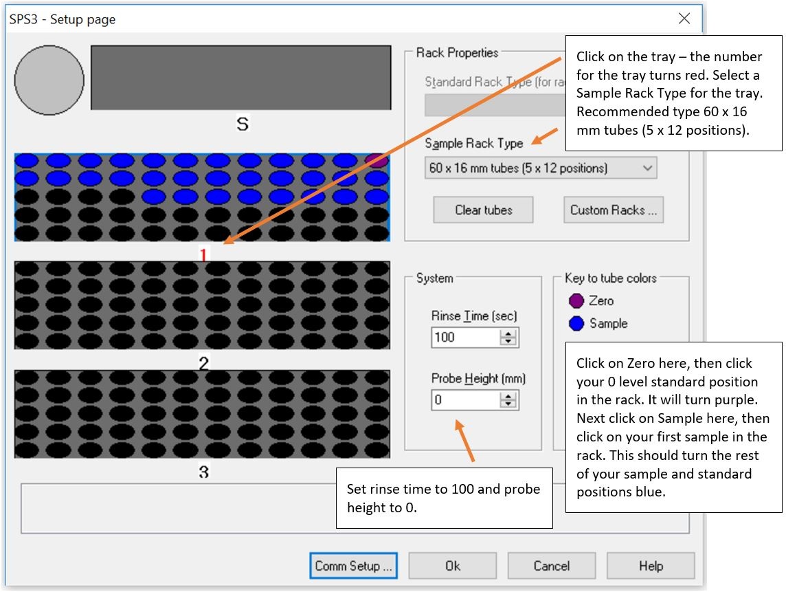
Figure 9 : Setup (Rinse/Rack type)
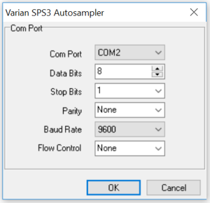
Figure 10 : Setup (Comm Setup/RS232 settings)
Click on Custom Racks (Figure 9) to configure sample racks.

Figure 11 : Setup (Custom Sample Rack Editor)
Running samples
- Prepare samples according to the protocol outlined in the above sections for the appropriate analyte.
- Click on START in the main Advanced Reads window (Figure 4).
- A window will pop-up showing the samples entered in the previous steps (Figure 12). Click OK.
- Save the data to a file for later viewing (Figure 13).
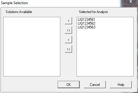
Figure 12 : Samples ready for analyses
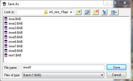
Figure 13 : Assigning a filename for the results
5. Observe where the samples need to go (Figure 14). Click OK.

Figure 14 : How to load the vials in the sample racks
6. View the results in real time (Figure 15).
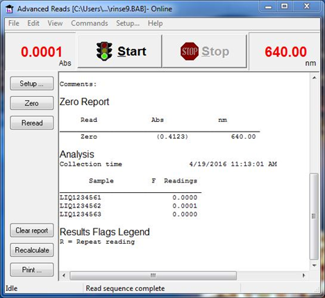
Figure 15 : Viewing results in real-time
7. Save the results to a .csv file.
- Select File → Export report (*.csv)
- Enter the location/file name.
8. Copy/paste into a calibration spreadsheet for manipulation and subsequent upload via Spreadsheet Uploader.
Using the results from the reads of the standards, create a calibration curve from the plot of the concentration vs. absorbance values. Use this equation to extrapolate the sample concentrations from their corresponding absorbance value. This can be done in the same spreadsheet as created above in the Advanced Reads application. This sheet can be loaded into the LIMS Spreadsheet Loader application as outlined in the LIMS Integration section.
Shutting down the Instrument
Aspirate approximately eight cycles of nanopure water, release the tubing on the peristaltic pump, turn off power to the unit and exit from the software. Clean any spills that may have occurred.
Empty the waste container and rinse with tap water.
QAQC
QA/QC for analysis consists of calibration verification using check standards, blanks and replicate samples.
QA/QC Types
Check Standard
A check standard for each set of analytes is run ~ every fifteen analyses depending on batch size. Check standards consist of a standard from approximately the midpoint of the calibration curve.
The check standard result is evaluated against the threshold for % variance limits for calibration verification standard against true value:
- Within ±10%: calibration is verified and sample analysis can continue.
- Outside of ±10%: check reagent solutions and rerun all samples in the corresponding analytical batch.
Blank
A blank is run with every batch to determine if high background levels are interfering with accurate sample results.
Replicate Samples
During each batch, a single sample should be run in duplicate and the variation of the results compared.
LIMS Integration
Results are stored in the LIMS database associated with an analysis code and an analysis component.
Analysis | Component Name | Component value | Unit |
SPEC | analyte | ammonium | NONE |
|
| phosphate | NONE |
|
| silica | NONE |
| concentration | concentration of analyte | µM |
Data collected is transferred to the LIMS database using IODP's Spreadsheet Loader application.
This is best done by entering the results into an Excel spreadsheet in a format similar to the pattern below, keeping the appropriate number of columns blank, and omitting the column headers.
Then run the Spreadsheet Loader application. Go to File > Load and it should import something like below (Figure 16).
To upload into the database, go to Lims > Upload and status messages will appear in the blank window.
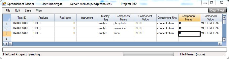
Figure 16 : Uploading results with Spreadsheet Uploader
Maintenance and Troubleshooting
Cleaning
Any spills in the sample compartment should be immediately wiped up and any deposits on the sample compartment windows should also be removed. The exterior surfaces should be cleaned with a soft cloth and, if necessary, this cloth can be dampened with water or a mild detergent.
Source Lamps
Instructions for how to change and align both the visible and UV lamps are included in the Help provided with the software. Care must be taken when removing lamps. Touching the glass envelope will reduce its efficiency. NEVER touch the glass surface of a new lamp. Always handle a lamp by its base, using a soft cloth.
Fuses
To replace a fuse, disconnect the unit from the power supply, and replace the blown fuse with one of the type and rating as outlined in the hardware specifications section.
- Disconnect the instrument from the power supply.
- Undo the fuse cap by pressing the cap and turning it counter-clockwise.
- Carefully pull out the cap. The fuse should be held in the fuse cap.
- Check that the fuse is the correct type and is not damaged. If necessary, replace it.
- Place the fuse into the cap, push the cap in and then turn the cap clockwise.
- Reconnect the instrument to the power supply.
Cary Win UV Help
Varian provides extensive help resources, available from the software CD. After installing the help utilities, go to START > All Programs > Varian > Cary WinUV > Cary Help.
Cary Help offers troubleshooting information, maintenance information like how to replace lamps, aligning lamps and mirrors, and replacing fuses and cleaning the flowcells.
Contact Information
Varian Instruments
1 800 926 3000
customer.service@varianinc.com
References
Gieskes, J.M., Gamo, T., and Brumsack, H., 1991. Chemical methods for interstitial water analysis aboard JOIDES Resolution, ODP Tech. Note, 15. doi:10.2973/odp.tn.15.1991.
Kastner, M., Elderfield, H., Martin, J.B., Suess, E., Kvenvolden, K.A., and Garrison, R.E., 1990. Diagenesis and interstitial water chemistry at the Peruvian margin—major constituents and strontium isotopes. In Suess, E., von Huene, R., et al., Proc. ODP, Sci. Results, 112: College Station, TX (Ocean Drilling Program), 413–440. doi:10.2973/odp.proc.sr.112.144.1990
Noriki, S. 1983. Silicate correction in the colorimetric determination of phosphate in seawater. J. Oceanograph. Soc. Japan, 39(6):324–326. doi:10.1007/BF02071829
Presley, B.J., 1971. Techniques for analyzing interstitial water samples: Appendix Part 1: determination of selected minor and major inorganic constituents. In Winterer, E.L., et al., Init. Repts. DSDP, 7(2): Washington, DC (U.S. Govt. Printing Office), 1749–1755. doi:10.2973/dsdp.proc.7.app1.1971
Solorzano, L., 1969. Determination of ammonia in natural waters by phenol-hypochlorite method. Limno. Oceanogr., 14:799–801.
Strickland, J.D.H., and Parsons, T.R., 1968. A manual for sea water analysis. Bull. Fish. Res. Board Can., 167.
Appendix
Hardware
The Varian Cary 100 is a double-beam, dual-chopper, monochromator UV-Vis spectrophotometer, centrally controlled by a PC. It has a high-performance R928 photomultiplier tube, tungsten halogen visible source with quartz window, and deuterium arc ultraviolet source.
Name | Agilent Technologies Cary UV-Vis Spectrophotometer |
Model | Cary-100 |
Serial number | UV1110M021 |
Dimensions | 26 × 26 × 13 in (unpacked) |
Weight | 99 lb (unpacked) |
Monochromator | Czerny-Turner 0.28 m |
Grating | 30 × 35 mm, 1200 lines/mm, blaze angle 8.6° at 240 nm |
Beam Splitting System | Chopper (30 Hz) |
Detectors | R928 PMT |
UV-Vis Limiting Resolution (nm) | 0.189 |
Wavelength Range (nm) | 190–900 |
Wavelength Accuracy (nm) | 0.02 at 656.1 nm; 0.04 at 486.0 nm |
Wavelength Reproducibility (nm) | 0.008 |
Signal Averaging (s) | 0.033–999 |
Spectral Bandwidth (nm) | 0.20–4.00 nm, 0.1 nm steps, motor driven |
Spectral Bandwidth Accuracy (nm) | @ 0.2: 0.193; @ 2.0: 2.03 |
Photometric Accuracy (Abs) | @ 0.3 Abs (Double Aperture method): 0.00016 |
Photometric Range (Abs) | 3.7 |
Photometric Display | (Abs) ± 9.9999; (%T) ± 200.00 |
Photometric Reproducibility | (Abs; NIST 930D filters) |
2 s signal averaging time @ 590 nm, 2 nm SBW |
|
2 s signal averaging time @ 546.1 nm, 2 nm SBW |
|
Photometric Stability (Abs/hr) | 2 h warmup |
Photometric Noise (Abs, RMS) | 2 nm SBW |
Baseline Flatness (Abs) | 0.00022 |
Sample Compartment Beam Separation (mm) | 110 |
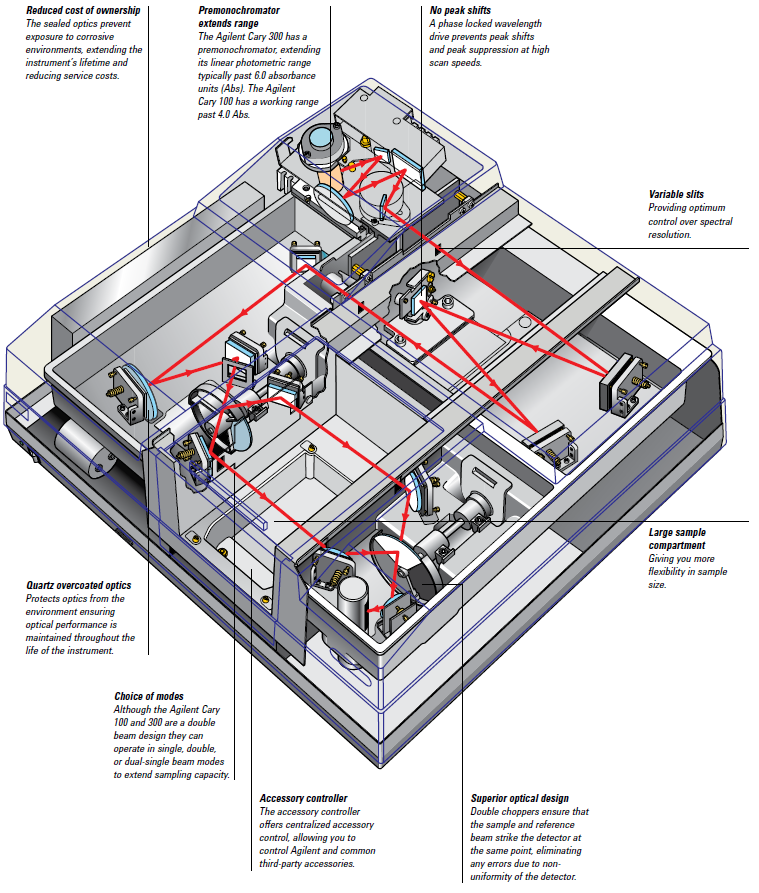
Figure 17 : Schematic of Cary Spectrophotometer
Electrical
Power supply (VAC) | 100, 120, 220, or 240 ± 10% |
Frequency (Hz) | 50 or 60 ± 1 with 400 VA power consumption |
Fuses (100–120 VAC) | T5 AH 250 V, IEC 127 sheet 5, 5 × 20 mm ceramic |
COM port (rear) | IEEE 488 |
PC port | USB |
Replacement Parts
Item | Part number |
Instrument fuse, 5 A time lag, ceramic, M205 | 1910009100 |
Peristaltic pump tubing replacement kit | 9910052900 |
Visible source lamp | 5610021700 |
Deuterium lamp | 5610021800 |
Dissolution cell, 715 µL, 10 mm | 6610015200 |
Thumbscrew kit | 9910064100 |
Spares kit: accessory locating pin, accessory fastening screws, instrument feet, instrument cover snap cap washer, snap cap, ACB cover plate, socket covers for ACB | 9910064300 |
Pumps
A double-action peristaltic pump services the feed and waste. 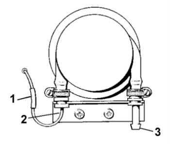
(1) plastic sleeve. (2) metal hook tubing. (3) waste outlet.
Credits
This document originated from Word documents Cary_UG_374_draft and CarySPS3_QSG_374_draft that were written by E. Moortgat (20111212). Credits for subsequent changes to this document are given in the page history.